Using callbacks in objectives¶

This notebook explains how to use a callback in an objective function. For details on the Callback class, see the API reference. Potential use cases for this are:

Plotting some outputs at each iteration of the optimization
Saving internal variables to plot once the optimization is complete

Some objectives have “internal callbacks” which are not intended to be user facing. These are standard callbacks that can be used to plot the results of an optimization by using DataFit.plot_fit_results(). For user-facing callbacks, users should create their own callback objects and call them directly for plotting, as demonstrated in this notebook.

Creating a custom callback¶

To implement a custom callback, create a class that inherits from iwp.callbacks.Callback and calls some specific functions. See the documentation for iwp.callbacks.Callback for more information on the available functions and their expected inputs.

import ionworkspipeline as iwp
import matplotlib.pyplot as plt
import pybamm
import numpy as np
import pandas as pd

class MyCallback(iwp.callbacks.Callback):
    def __init__(self):
        super().__init__()
        # Implement our own iteration counter
        self.iter = 0

    def on_objective_build(self, logs):
        self.data_ = logs["data"]

    def on_run_iteration(self, logs):
        # Print some information at each iteration
        inputs = logs["inputs"]
        V_model = logs["outputs"]["Voltage [V]"]
        V_data = self.data_["Voltage [V]"]

        # calculate RMSE, note this is not necessarily the cost function used in the optimization
        rmse = np.sqrt(np.nanmean((V_model - V_data) ** 2))

        print(f"Iteration: {self.iter}, Inputs: {inputs}, RMSE: {rmse}")
        self.iter += 1

    def on_datafit_finish(self, logs):
        self.fit_results_ = logs

    def plot_fit_results(self):
        """
        Plot the fit results.
        """
        data = self.data_
        fit = self.fit_results_["outputs"]

        fit_results = {
            "data": (data["Time [s]"], data["Voltage [V]"]),
            "fit": (fit["Time [s]"], fit["Voltage [V]"]),
        }

        markers = {"data": "o", "fit": "--"}
        colors = {"data": "k", "fit": "tab:red"}
        fig, ax = plt.subplots()
        for name, (t, V) in fit_results.items():
            ax.plot(
                t,
                V,
                markers[name],
                label=name,
                color=colors[name],
                mfc="none",
                linewidth=2,
            )
        ax.grid(alpha=0.5)
        ax.set_xlabel("Time [s]")
        ax.set_ylabel("Voltage [V]")
        ax.legend()

        return fig, ax

To use this callback, we generate synthetic data for a current-driven experiment and fit a SPM using the CurrentDriven objective.

model = pybamm.lithium_ion.SPM()
parameter_values = pybamm.ParameterValues("Chen2020")
t = np.linspace(0, 3600, 1000)
sim = iwp.Simulation(model, parameter_values=parameter_values, t_eval=t, t_interp=t)
sim.solve()
data = pd.DataFrame(
    {x: sim.solution[x].entries for x in ["Time [s]", "Current [A]", "Voltage [V]"]}
)

# In this example we just fit the diffusivity in the positive electrode
parameters = {
    "Positive particle diffusivity [m2.s-1]": iwp.Parameter("D_s", initial_value=1e-15),
}

# Create the callback
callback = MyCallback()
objective = iwp.objectives.CurrentDriven(
    data, options={"model": model}, callbacks=callback
)
current_driven = iwp.DataFit(objective, parameters=parameters)

# make sure we're not accidentally initializing with the correct values by passing
# them in
params_for_pipeline = {k: v for k, v in parameter_values.items() if k not in parameters}

_ = current_driven.run(params_for_pipeline)

Iteration: 0, Inputs: {'D_s': 1.0}, RMSE: 0.15909623872027936
Iteration: 1, Inputs: {'D_s': 1.0}, RMSE: 0.15909623872027936
Iteration: 2, Inputs: {'D_s': 2.0}, RMSE: 0.06447715147661243
Iteration: 3, Inputs: {'D_s': 0.0}, RMSE: 9999999996.444777
Iteration: 4, Inputs: {'D_s': 1.500000000015711}, RMSE: 0.10181491876740152

[IDAS ERROR]  IDASolve
  At t = 0 and h = 8.88113e-60, the corrector convergence failed repeatedly or with |h| = hmin.

Iteration: 5, Inputs: {'D_s': 2.25}, RMSE: 0.05119216091537602
Iteration: 6, Inputs: {'D_s': 2.35}, RMSE: 0.04656550635497967
Iteration: 7, Inputs: {'D_s': 2.45}, RMSE: 0.04225747901602169
Iteration: 8, Inputs: {'D_s': 2.5500000000000003}, RMSE: 0.0382369172532095
Iteration: 9, Inputs: {'D_s': 2.6500000000000004}, RMSE: 0.034473436302257555
Iteration: 10, Inputs: {'D_s': 2.79142135623731}, RMSE: 0.02954660806680908
Iteration: 11, Inputs: {'D_s': 2.89142135623731}, RMSE: 0.026302653676810863
Iteration: 12, Inputs: {'D_s': 2.99142135623731}, RMSE: 0.023247876819624265
Iteration: 13, Inputs: {'D_s': 3.13284271247462}, RMSE: 0.01921256061607784
Iteration: 14, Inputs: {'D_s': 3.33284271247462}, RMSE: 0.01401280229847055
Iteration: 15, Inputs: {'D_s': 3.43284271247462}, RMSE: 0.011610464755135651
Iteration: 16, Inputs: {'D_s': 3.5328427124746202}, RMSE: 0.009326575370641268
Iteration: 17, Inputs: {'D_s': 3.67426406871193}, RMSE: 0.0062833537305494735

Iteration: 18, Inputs: {'D_s': 3.827353984261646}, RMSE: 0.003212959555045286
Iteration: 19, Inputs: {'D_s': 3.927353984261646}, RMSE: 0.0013219099027846316
Iteration: 20, Inputs: {'D_s': 4.027353984261646}, RMSE: 0.0004853044688969927
Iteration: 21, Inputs: {'D_s': 4.168775340498955}, RMSE: 0.0029058988941809737
Iteration: 22, Inputs: {'D_s': 4.092118921614875}, RMSE: 0.0016110869070794871
Iteration: 23, Inputs: {'D_s': 4.055618610271941}, RMSE: 0.000979193838296977
Iteration: 24, Inputs: {'D_s': 4.002353984261646}, RMSE: 4.172274185303044e-05
Iteration: 25, Inputs: {'D_s': 3.977353984261646}, RMSE: 0.00040826019467569714
Iteration: 26, Inputs: {'D_s': 4.012353984261646}, RMSE: 0.0002194391590760842
Iteration: 27, Inputs: {'D_s': 3.992353984261646}, RMSE: 0.00013826179083376082
Iteration: 28, Inputs: {'D_s': 4.007301201264901}, RMSE: 0.00012954888582715878
Iteration: 29, Inputs: {'D_s': 3.999853984261646}, RMSE: 8.41311869369533e-06
Iteration: 30, Inputs: {'D_s': 4.004822665481068}, RMSE: 8.54512245756432e-05
Iteration: 31, Inputs: {'D_s': 4.0013539842616455}, RMSE: 2.4364576712400924e-05

Iteration: 32, Inputs: {'D_s': 4.000353984261645}, RMSE: 9.229043958530913e-06
Iteration: 33, Inputs: {'D_s': 3.998939770699272}, RMSE: 2.1405422417413923e-05
Iteration: 34, Inputs: {'D_s': 4.000853214099611}, RMSE: 1.6097265986298933e-05
Iteration: 35, Inputs: {'D_s': 4.000103984261645}, RMSE: 7.612978769392109e-06
Iteration: 36, Inputs: {'D_s': 3.999896955722756}, RMSE: 8.108001486560992e-06
Iteration: 37, Inputs: {'D_s': 4.000203984261645}, RMSE: 8.002941820134204e-06
Iteration: 38, Inputs: {'D_s': 4.000003984261645}, RMSE: 7.636885061957086e-06
Iteration: 39, Inputs: {'D_s': 4.000153983098626}, RMSE: 7.759029445196987e-06
Iteration: 40, Inputs: {'D_s': 4.000078984261645}, RMSE: 7.582382501770634e-06
Iteration: 41, Inputs: {'D_s': 4.000128983598464}, RMSE: 7.673335487947358e-06
Iteration: 42, Inputs: {'D_s': 4.000093984261645}, RMSE: 7.599905484623462e-06
Iteration: 43, Inputs: {'D_s': 4.000113984261644}, RMSE: 7.634037512953642e-06
Iteration: 44, Inputs: {'D_s': 4.000108984255365}, RMSE: 7.6229908840228175e-06
Iteration: 45, Inputs: {'D_s': 4.000101484261645}, RMSE: 7.608361932179118e-06

Iteration: 46, Inputs: {'D_s': 4.000098984261645}, RMSE: 7.60400522015036e-06
Iteration: 47, Inputs: {'D_s': 4.000095448727739}, RMSE: 7.598288825977144e-06
Iteration: 48, Inputs: {'D_s': 4.00009044872774}, RMSE: 7.594925227573238e-06
Iteration: 49, Inputs: {'D_s': 4.0000929487277395}, RMSE: 7.598392635776437e-06
Iteration: 50, Inputs: {'D_s': 4.0000972164943285}, RMSE: 7.601081802450524e-06
Iteration: 51, Inputs: {'D_s': 4.000094448727739}, RMSE: 7.600598604717619e-06
Iteration: 52, Inputs: {'D_s': 4.000096332610969}, RMSE: 7.599669000587468e-06
Iteration: 53, Inputs: {'D_s': 4.000095448727739}, RMSE: 7.598288825977144e-06

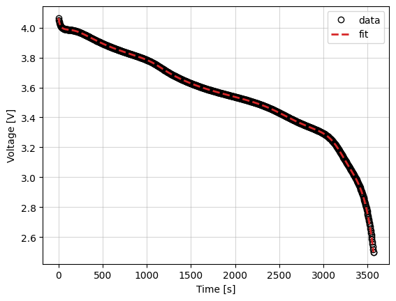
Now we use the callback object we created to plot the results at the end of the optimization.

_ = callback.plot_fit_results()

../../../_images/1ed99dec172060bbaef520ec2f24e63fa26fe132af809557d68422af3cb533c4.png

Cost logger¶

The DataFit class has an internal “cost-logger” attribute that can be used to log and visualize the cost function during optimization. This is useful for monitoring the progress of the optimization. The cost logger is a dictionary that stores the cost function value at each iteration. The cost logger can be accessed using the cost_logger attribute of the DataFit object.

By default, the cost logger tracks the cost function value. DataFit.plot_trace can be used the plot the progress at the end of the optimization.

objective = iwp.objectives.CurrentDriven(data, options={"model": model})
current_driven = iwp.DataFit(objective, parameters=parameters)
_ = current_driven.run(params_for_pipeline)
_ = current_driven.plot_trace()

[IDAS ERROR]  IDASolve
  At t = 0 and h = 8.88113e-60, the corrector convergence failed repeatedly or with |h| = hmin.

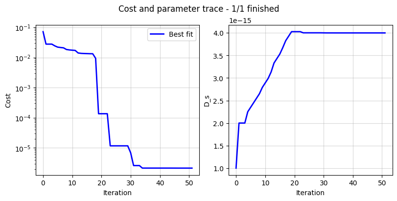
../../../_images/f6a2b34a79d55200859629e5364f5a8b894d33f20136d9c9c93cb718d4117dae.png

The cost logger can be changed by passing the cost_logger argument to the DataFit object. For example, the following example shows how to pass a cost logger that plots the cost function and parameter values every 10 seconds.

current_driven = iwp.DataFit(
    objective,
    parameters=parameters,
    cost_logger=iwp.data_fits.CostLogger(plot_every=10),
)