Using callbacks in objectives

This notebook explains how to use a callback in an objective function. For details on the Callback class, see the API reference. Potential use cases for this are:

• Plotting some outputs at each iteration of the optimization

• Saving internal variables to plot once the optimization is complete

Some objectives have “internal callbacks” which are not intended to be user facing. These are standard callbacks that can be used to plot the results of an optimization by using DataFit.plot_fit_results(). For user-facing callbacks, users should create their own callback objects and call them directly for plotting, as demonstrated in this notebook.

Creating a custom callback

To implement a custom callback, create a class that inherits from iwp.callbacks.Callback and calls some specific functions. See the documentation for iwp.callbacks.Callback for more information on the available functions and their expected inputs.

import ionworkspipeline as iwp
import matplotlib.pyplot as plt
import pybamm
import numpy as np
import pandas as pd

class MyCallback(iwp.callbacks.Callback):
    def __init__(self):
        super().__init__()
        # Implement our own iteration counter
        self.iter = 0

    def on_objective_build(self, logs):
        self.data_ = logs["data"]

    def on_run_iteration(self, logs):
        # Print some information at each iteration
        inputs = logs["inputs"]
        V_model = logs["outputs"]["Voltage [V]"]
        V_data = self.data_["Voltage [V]"]

        # calculate RMSE, note this is not necessarily the cost function used in the optimization
        rmse = np.sqrt(np.nanmean((V_model - V_data) ** 2))

        print(f"Iteration: {self.iter}, Inputs: {inputs}, RMSE: {rmse}")
        self.iter += 1

    def on_datafit_finish(self, logs):
        self.fit_results_ = logs

    def plot_fit_results(self):
        """
        Plot the fit results.
        """
        data = self.data_
        fit = self.fit_results_["outputs"]

        fit_results = {
            "data": (data["Time [s]"], data["Voltage [V]"]),
            "fit": (fit["Time [s]"], fit["Voltage [V]"]),
        }

        markers = {"data": "o", "fit": "--"}
        colors = {"data": "k", "fit": "tab:red"}
        fig, ax = plt.subplots()
        for name, (t, V) in fit_results.items():
            ax.plot(
                t,
                V,
                markers[name],
                label=name,
                color=colors[name],
                mfc="none",
                linewidth=2,
            )
        ax.grid(alpha=0.5)
        ax.set_xlabel("Time [s]")
        ax.set_ylabel("Voltage [V]")
        ax.legend()

        return fig, ax

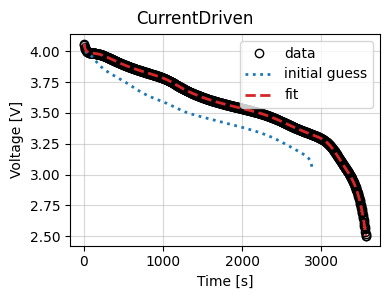
To use this callback, we generate synthetic data for a current-driven experiment and fit a SPM using the CurrentDriven objective.

model = pybamm.lithium_ion.SPM()
parameter_values = iwp.ParameterValues("Chen2020")
t = np.linspace(0, 3600, 1000)
sim = iwp.Simulation(model, parameter_values=parameter_values, t_eval=t, t_interp=t)
sim.solve()
data = pd.DataFrame(
    {x: sim.solution[x].entries for x in ["Time [s]", "Current [A]", "Voltage [V]"]}
)

# In this example we just fit the diffusivity in the positive electrode
parameters = {
    "Positive particle diffusivity [m2.s-1]": iwp.Parameter("D_s", initial_value=1e-15),
}

# Create the callback
callback = MyCallback()
objective = iwp.objectives.CurrentDriven(
    data, options={"model": model}, callbacks=callback
)
current_driven = iwp.DataFit(objective, parameters=parameters)

# make sure we're not accidentally initializing with the correct values by passing
# them in
params_for_pipeline = {k: v for k, v in parameter_values.items() if k not in parameters}

results = current_driven.run(params_for_pipeline)

Iteration: 0, Inputs: {'D_s': 1.0}, RMSE: 0.15909623870900977
Iteration: 1, Inputs: {'D_s': 1.0}, RMSE: 0.15909623870900977
Iteration: 2, Inputs: {'D_s': 2.0}, RMSE: 0.06447715147451864
Iteration: 3, Inputs: {'D_s': 0.0}, RMSE: 9999999996.444777
Iteration: 4, Inputs: {'D_s': 1.5000000000000018}, RMSE: 0.10181491874614104
Iteration: 5, Inputs: {'D_s': 2.25}, RMSE: 0.05119216091391999
Iteration: 6, Inputs: {'D_s': 2.5}, RMSE: 0.040213641940608925
Iteration: 7, Inputs: {'D_s': 2.6}, RMSE: 0.03632444183138642
Iteration: 8, Inputs: {'D_s': 2.5}, RMSE: 0.040213641940608925
Iteration: 9, Inputs: {'D_s': 2.7}, RMSE: 0.03267971456003209
Iteration: 10, Inputs: {'D_s': 2.8000000000000003}, RMSE: 0.029260996684279166
Iteration: 11, Inputs: {'D_s': 2.9000000000000004}, RMSE: 0.02603357723998981
Iteration: 12, Inputs: {'D_s': 3.0000000000000004}, RMSE: 0.022993913200343732
Iteration: 13, Inputs: {'D_s': 3.14142135623731}, RMSE: 0.01897786533455976
Iteration: 14, Inputs: {'D_s': 3.3414213562373103}, RMSE: 0.013801829369504458
Iteration: 15, Inputs: {'D_s': 3.4414213562373104}, RMSE: 0.011410032929092205
Iteration: 16, Inputs: {'D_s': 3.5414213562373105}, RMSE: 0.00913591889127036

[IDAS ERROR]  IDASolve
  At t = 0 and h = 1e-09, the corrector convergence failed repeatedly or with |h| = hmin.

Iteration: 17, Inputs: {'D_s': 3.68284271247462}, RMSE: 0.006105359639542874
Iteration: 18, Inputs: {'D_s': 3.8255560283241605}, RMSE: 0.003247758708932552
Iteration: 19, Inputs: {'D_s': 3.9255560283241606}, RMSE: 0.0013551503633464908
Iteration: 20, Inputs: {'D_s': 4.025556028324161}, RMSE: 0.0004535256628975395
Iteration: 21, Inputs: {'D_s': 4.12555602832416}, RMSE: 0.002181173029465835
Iteration: 22, Inputs: {'D_s': 4.0751525550821075}, RMSE: 0.001318622201698045
Iteration: 23, Inputs: {'D_s': 4.00055602832416}, RMSE: 1.1678128222598267e-05
Iteration: 24, Inputs: {'D_s': 3.9905560283241606}, RMSE: 0.00017050656583187017
Iteration: 25, Inputs: {'D_s': 4.01055602832416}, RMSE: 0.00018746623849406134
Iteration: 26, Inputs: {'D_s': 4.005555716999232}, RMSE: 9.848790651845809e-05
Iteration: 27, Inputs: {'D_s': 3.9980560283241604}, RMSE: 3.6630974734461494e-05
Iteration: 28, Inputs: {'D_s': 4.003055856717626}, RMSE: 5.410125269855649e-05
Iteration: 29, Inputs: {'D_s': 3.9995560283241605}, RMSE: 1.1757845383911372e-05
Iteration: 30, Inputs: {'D_s': 4.001556028324161}, RMSE: 2.7819953964617322e-05
Iteration: 31, Inputs: {'D_s': 4.0010560277573015}, RMSE: 1.9372530766331914e-05
Iteration: 32, Inputs: {'D_s': 4.00030602832416}, RMSE: 8.766723703500031e-06
Iteration: 33, Inputs: {'D_s': 4.000058436588003}, RMSE: 7.5737564934194014e-06
Iteration: 34, Inputs: {'D_s': 4.00040602832416}, RMSE: 9.791248288946835e-06

Iteration: 35, Inputs: {'D_s': 4.00020602832416}, RMSE: 8.014878054710695e-06
Iteration: 36, Inputs: {'D_s': 4.0001060283241605}, RMSE: 7.616946572852944e-06
Iteration: 37, Inputs: {'D_s': 4.000058781983221}, RMSE: 7.573754188003006e-06
Iteration: 38, Inputs: {'D_s': 4.0001310283241605}, RMSE: 7.679402910161566e-06
Iteration: 39, Inputs: {'D_s': 4.000118528324105}, RMSE: 7.644970332010601e-06
Iteration: 40, Inputs: {'D_s': 4.000096028324161}, RMSE: 7.599190176954692e-06
Iteration: 41, Inputs: {'D_s': 4.000086028324161}, RMSE: 7.589435237500911e-06
Iteration: 42, Inputs: {'D_s': 4.000101028324158}, RMSE: 7.607547969713152e-06
Iteration: 43, Inputs: {'D_s': 4.000093528324161}, RMSE: 7.5992338637845886e-06
Iteration: 44, Inputs: {'D_s': 4.000098528324159}, RMSE: 7.603238746280279e-06
Iteration: 45, Inputs: {'D_s': 4.000095028324161}, RMSE: 7.5976438263492404e-06
Iteration: 46, Inputs: {'D_s': 4.000094028324161}, RMSE: 7.599970851947887e-06
Iteration: 47, Inputs: {'D_s': 4.000095028324161}, RMSE: 7.5976438263492404e-06

Now we use the results to plot the fit at the end of the optimization.

_ = results.plot_fit_results()

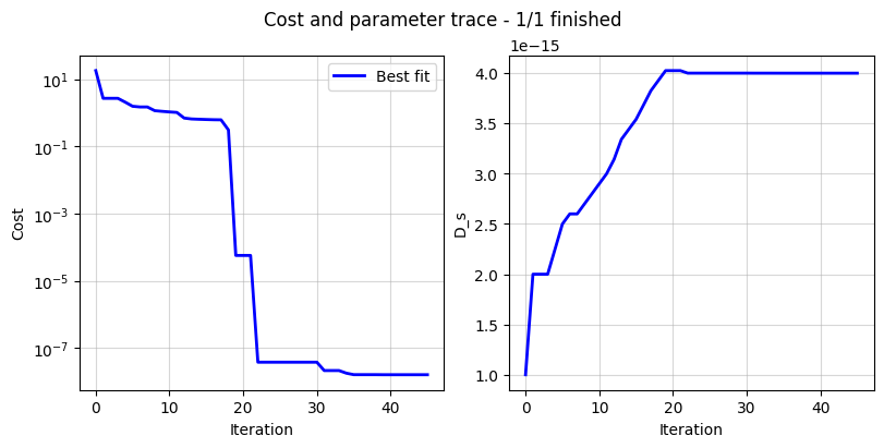
Cost logger

The DataFit class has an internal “cost-logger” attribute that can be used to log and visualize the cost function during optimization. This is useful for monitoring the progress of the optimization. The cost logger is a dictionary that stores the cost function value at each iteration. The cost logger can be accessed using the cost_logger attribute of the DataFit object.

By default, the cost logger tracks the cost function value. DataFit.plot_trace can be used the plot the progress at the end of the optimization.

objective = iwp.objectives.CurrentDriven(data, options={"model": model})
current_driven = iwp.DataFit(objective, parameters=parameters)
_ = current_driven.run(params_for_pipeline)
_ = current_driven.plot_trace()

[IDAS ERROR]  IDASolve
  At t = 0 and h = 1e-09, the corrector convergence failed repeatedly or with |h| = hmin.

The cost logger can be changed by passing the cost_logger argument to the DataFit object. For example, the following example shows how to pass a cost logger that plots the cost function and parameter values every 10 seconds.

current_driven = iwp.DataFit(
    objective,
    parameters=parameters,
    cost_logger=iwp.data_fits.CostLogger(plot_every=10),
)