3. Half-cell GITT

In this example, we fit the exchange current density and diffusivity for the half-cells using synthetic GITT data. We use the half-cell MSMR functions fitted and saved in half-cell OCP notebook to create interpolants for the OCP as a function of stoichiometry.

Before running this example, make sure to run the script true_parameters/generate_data.py to generate the synthetic data.

from pathlib import Path
import ionworkspipeline as iwp
import pandas as pd
import json
import pybamm
import iwutil

from plots import constant_current, drive_cycle
from true_parameters.parameters import half_cell

iwp.set_logging_level("INFO")

We begin by making a list of “known parameters”. These are values that are already known from other sources (e.g. spec sheet, direct measurement, other experiments). For this example we load the known parameters from the true parameters used to generate the synthetic data.

# list of parameters that are known (in practice these would be collected from a data
# sheet or from additional experimental measurements)
KNOWN_PARAMETERS = [
    # Separator
    "Separator thickness [m]",
    "Separator porosity",
    # Positive electrode
    "Positive electrode thickness [m]",
    "Positive electrode conductivity [S.m-1]",
    "Positive electrode porosity",
    "Positive electrode active material volume fraction",
    "Positive particle radius [m]",
    "Positive electrode OCP entropic change [V.K-1]",
    # Cell
    "Electrode height [m]",
    "Electrode width [m]",
    # these are user-specified at the cell level and may differ from the actual
    # voltage and capacity as measured in the experiment
    "Lower voltage cut-off [V]",
    "Upper voltage cut-off [V]",
    "Open-circuit voltage at 0% SOC [V]",
    "Open-circuit voltage at 100% SOC [V]",
    "Nominal cell capacity [A.h]",
    "Current function [A]",
]

Next, we create a function to fit the exchange current density and diffusivity for the half-cells using the synthetic GITT data for each electrode.

The function begins by loading in the known parameter values and previously fitted parameters. It then loads in the data and sets up the objective function for the GITT experiment. Next we set up the objective function for the GITT experiment. In order to do this, we first split the data into cycles, then for each pulse we set up a Pulse objective, which takes in the data and some extra options, including the model to use for the fitting. We set this up using the get_pulse_objectives_by_cycle function. This returns a dictionary of PulseHalfCell objectives with keys corresponding to the cycle number. We pass the dictionary to the DataFit object, which will fit the parameters simultaneously across all objectives in the dictionary.

We then set up the iwp.Parameter objects and functional form for any functions – here we use a symmetric exchange-current density and scalar diffusivity.

Finally the calculations and fits are put together in a pipeline. The pipeline takes in the known and previously calculated parameters, constructs an interpolant for the OCP, performs electrode State of Health calculations to get the minimum and maximum stoichiometries, and fits the exchange-current density and diffusivity for each electrode. The results are saved to a file.

def fit_save(electrode, cycles_to_use=None):
    # Load true parameters from which we will read in the "known" values
    true_parameter_values = pybamm.ParameterValues(half_cell(electrode))
    known_parameter_values = {k: true_parameter_values[k] for k in KNOWN_PARAMETERS}
    known_values = iwp.direct_entries.DirectEntry(
        known_parameter_values, "Measured or assumed values"
    )

    # Read in previously fitted OCP parameters
    # Note: PyBaMM expects the working electrode to be positive
    ocp = iwp.calculations.ocp_data_interpolant_from_csv(
        "positive",
        f"fitted_parameters/{electrode}_electrode_ocp.csv",
    )
    with open(f"fitted_parameters/{electrode}_electrode_ocp.json") as f:
        ocp_params = json.load(f)
    if electrode == "negative":
        ocp_params = iwp.data_fits.util.negative_to_positive_half_cell(ocp_params)
    Q_total = ocp_params["Half-cell positive electrode capacity [A.h]"]
    ocp_params.update(
        {
            "Positive electrode capacity [A.h]": Q_total,
        }
    )
    ocp_params = iwp.direct_entries.DirectEntry(ocp_params, "Fitted OCP parameters")

    # Load GITT data
    gitt_data = pd.read_csv(
        Path("synthetic_data") / f"half_cell_{electrode}_electrode" / "gitt.csv"
    )
    if cycles_to_use is not None:
        gitt_data = gitt_data[gitt_data["Cycle number"].isin(cycles_to_use)]

    # Set up parameters to fit
    def j0_half_cell(c_e, c_s_surf, c_s_max, T):
        j0_ref = pybamm.Parameter(
            "Positive electrode reference exchange-current density [A.m-2]"
        )
        alpha = 0.5
        c_e_ref = 1000

        return (
            j0_ref
            * (c_e / c_e_ref) ** (1 - alpha)
            * (c_s_surf / c_s_max) ** alpha
            * (1 - c_s_surf / c_s_max) ** (1 - alpha)
        )

    gitt_params = {
        "Positive electrode exchange-current density [A.m-2]": j0_half_cell,
        "Positive electrode reference exchange-current density [A.m-2]": iwp.Parameter(
            "Positive electrode exchange-current density [A.m-2]", bounds=(0.1, 100)
        ),
        "Positive particle diffusivity [m2.s-1]": iwp.Parameter(
            "Positive particle diffusivity [m2.s-1]",
            initial_value=1e-14,
            bounds=(1e-15, 1e-13),
        ),
    }

    # Make data fit - we construct objectives for each GITT pulse and fit across
    # all of them simultaneously
    model = pybamm.lithium_ion.SPMe({"working electrode": "positive"})
    solver = pybamm.IDAKLUSolver()
    objectives = iwp.objectives.pulse.get_pulse_objectives_by_cycle(
        gitt_data,
        options={"model": model, "solver": solver},
    )
    gitt = iwp.DataFit(
        objectives,
        parameters=gitt_params,
    )

    # Construct pipeline
    initial_soc = 1
    pipeline = iwp.Pipeline(
        {
            **iwp.pipelines.half_cell.defaults(),
            "known values": known_values,
            "OCP interpolant": ocp,
            "OCP parameters": ocp_params,
            "maximum concentration": iwp.calculations.ElectrodeCapacity(
                "positive",
                unknown="maximum concentration",
                method="capacity",
            ),
            "electrode SOH calculations": iwp.calculations.ElectrodeSOHHalfCell(
                "positive"
            ),
            "initial concentration": iwp.calculations.InitialSOCHalfCell(
                "positive", initial_soc
            ),
            "GITT": gitt,
        },
    )

    # Run pipeline
    fitted_parameter_values = pipeline.run()

    # Save parameters to JSON
    params_to_save = {
        f"{electrode.capitalize()} electrode reference exchange-current density [A.m-2]": fitted_parameter_values[
            "Positive electrode reference exchange-current density [A.m-2]"
        ],
        f"{electrode.capitalize()} particle diffusivity [m2.s-1]": fitted_parameter_values[
            "Positive particle diffusivity [m2.s-1]"
        ],
    }
    iwutil.save.json(
        params_to_save,
        Path("fitted_parameters") / f"{electrode}_electrode_gitt.json",
    )

    # Export a .py file with the PyBaMM parameters
    # Note: if we specify data_path=None, the variable DATA_PATH will be set to the
    # directory containing the exported script
    iwp.util.export_python_script(
        fitted_parameter_values,
        f"fitted_parameters/{electrode}_half_cell.py",
        data_path=None,
    )
    return pipeline, fitted_parameter_values

We run the fit for each electrode, storing the results in a dictionary.

Note: in the interest of speeding up the example, we just perform the fit on a few cycles of the GITT data. In practice, you would want to use the entire dataset.

cycles_to_use = [1, 2, 3, 4, 5]

pipelines = {}
fitted_parameter_values = {}
for electrode in ["negative", "positive"]:
    pipelines[electrode], fitted_parameter_values[electrode] = fit_save(
        electrode, cycles_to_use=cycles_to_use
    )

2024-11-08 20:14:05.158 - [INFO] pipeline.run(122): Running 'defaults' component (Standard defaults for parameters that are not explicitly set by the user)

2024-11-08 20:14:05.159 - [INFO] pipeline.run(122): Running 'Bruggeman' component (Bruggeman coefficients, defaulting to 1.5 for electrolyte and 0 for electrode)

2024-11-08 20:14:05.160 - [INFO] pipeline.run(122): Running 'temperatures' component (All 'temperature' parameters set to 298.15 [K])

2024-11-08 20:14:05.161 - [INFO] pipeline.run(122): Running 'lithium metal anode' component (Parameters for a generic lithium metal counter electrode with parameter values that don't add any overpotential)

2024-11-08 20:14:05.162 - [INFO] pipeline.run(122): Running 'electrolyte' component (Electrolyte parameters from Nyman et al. (2008) with initial electrolyte concentration set to 1000 [mol.m-3])

2024-11-08 20:14:05.163 - [INFO] pipeline.run(122): Running 'known values' component (Measured or assumed values)

2024-11-08 20:14:05.164 - [INFO] pipeline.run(122): Running 'OCP interpolant' component (Create interpolant for OCP from data)

2024-11-08 20:14:05.166 - [INFO] pipeline.run(122): Running 'OCP parameters' component (Fitted OCP parameters)

2024-11-08 20:14:05.166 - [INFO] pipeline.run(122): Running 'maximum concentration' component (Calculation of maximum concentration from the other variables related to electrode capacity, for the positive electrode using the capacity capacity)

2024-11-08 20:14:05.181 - [INFO] pipeline.run(122): Running 'electrode SOH calculations' component (Calculation of minimum and maximum stoichiometries in the positive electrode from capacity)

2024-11-08 20:14:05.222 - [INFO] pipeline.run(122): Running 'initial concentration' component (Initial concentration for a target SOC)

2024-11-08 20:14:05.223 - [INFO] pipeline.run(122): Running 'GITT' component ()

2024-11-08 20:14:54.863 - [INFO] pipeline.run(122): Running 'defaults' component (Standard defaults for parameters that are not explicitly set by the user)

2024-11-08 20:14:54.864 - [INFO] pipeline.run(122): Running 'Bruggeman' component (Bruggeman coefficients, defaulting to 1.5 for electrolyte and 0 for electrode)

2024-11-08 20:14:54.865 - [INFO] pipeline.run(122): Running 'temperatures' component (All 'temperature' parameters set to 298.15 [K])

2024-11-08 20:14:54.866 - [INFO] pipeline.run(122): Running 'lithium metal anode' component (Parameters for a generic lithium metal counter electrode with parameter values that don't add any overpotential)

2024-11-08 20:14:54.867 - [INFO] pipeline.run(122): Running 'electrolyte' component (Electrolyte parameters from Nyman et al. (2008) with initial electrolyte concentration set to 1000 [mol.m-3])

2024-11-08 20:14:54.868 - [INFO] pipeline.run(122): Running 'known values' component (Measured or assumed values)

2024-11-08 20:14:54.869 - [INFO] pipeline.run(122): Running 'OCP interpolant' component (Create interpolant for OCP from data)

2024-11-08 20:14:54.870 - [INFO] pipeline.run(122): Running 'OCP parameters' component (Fitted OCP parameters)

2024-11-08 20:14:54.871 - [INFO] pipeline.run(122): Running 'maximum concentration' component (Calculation of maximum concentration from the other variables related to electrode capacity, for the positive electrode using the capacity capacity)

2024-11-08 20:14:54.884 - [INFO] pipeline.run(122): Running 'electrode SOH calculations' component (Calculation of minimum and maximum stoichiometries in the positive electrode from capacity)

2024-11-08 20:14:54.925 - [INFO] pipeline.run(122): Running 'initial concentration' component (Initial concentration for a target SOC)

2024-11-08 20:14:54.926 - [INFO] pipeline.run(122): Running 'GITT' component ()

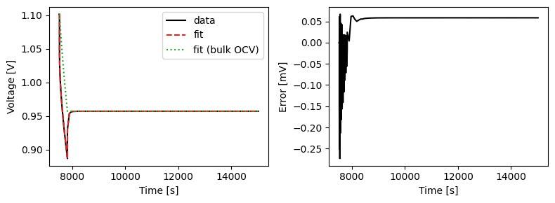
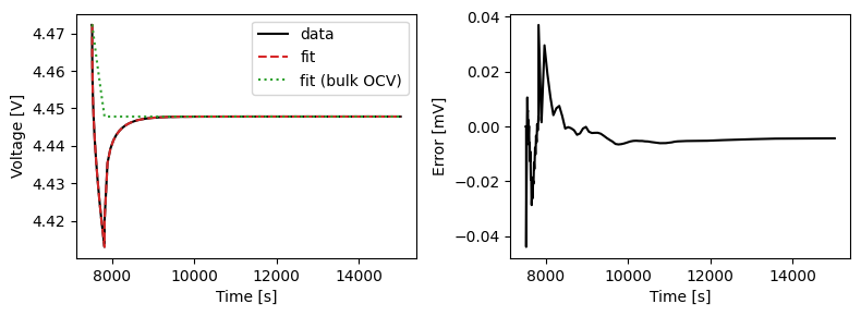
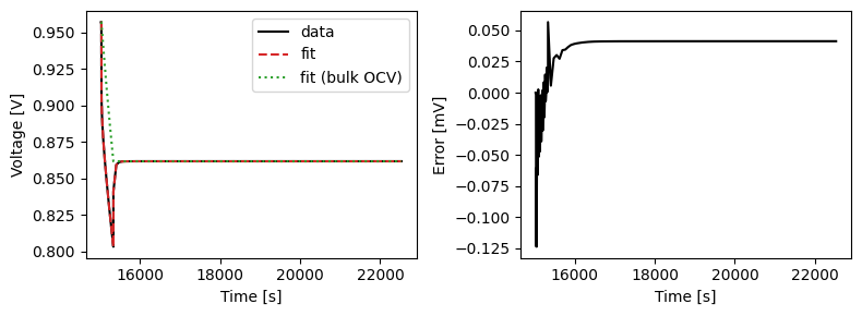
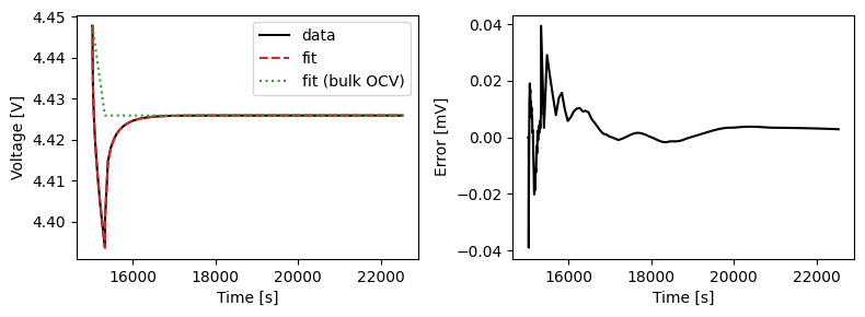
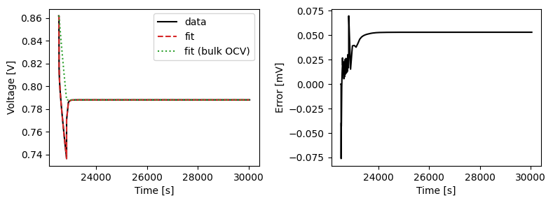
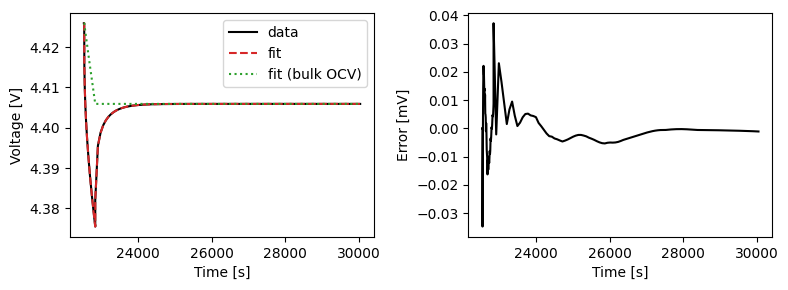
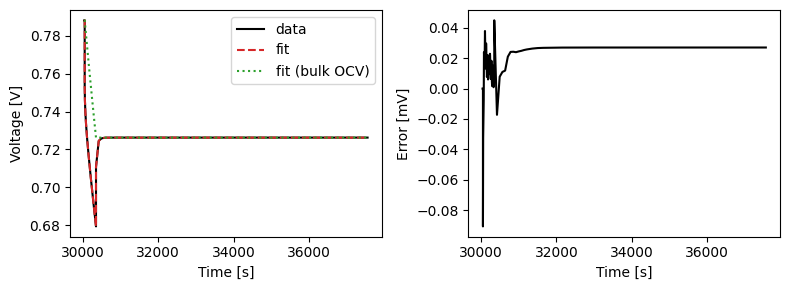
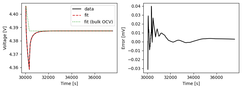
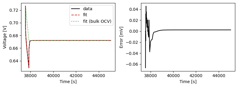
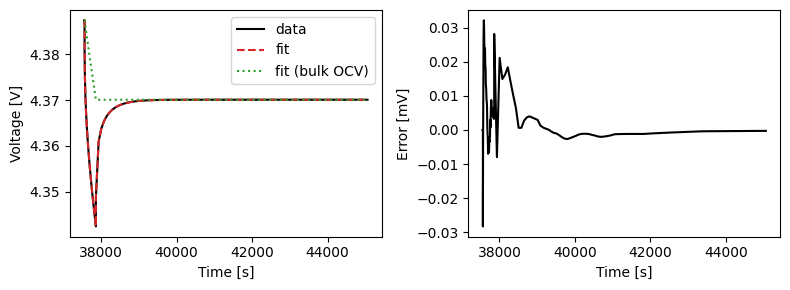
We can plot the results of the GITT fit by indexing into the objectives using the cycle number and plotting the fit results from the callback. Let’s plot a few as an example.

for cycle in cycles_to_use:
    pipelines["negative"].components["GITT"].objectives[cycle].callbacks[
        0
    ].plot_fit_results()
    pipelines["positive"].components["GITT"].objectives[cycle].callbacks[
        0
    ].plot_fit_results()

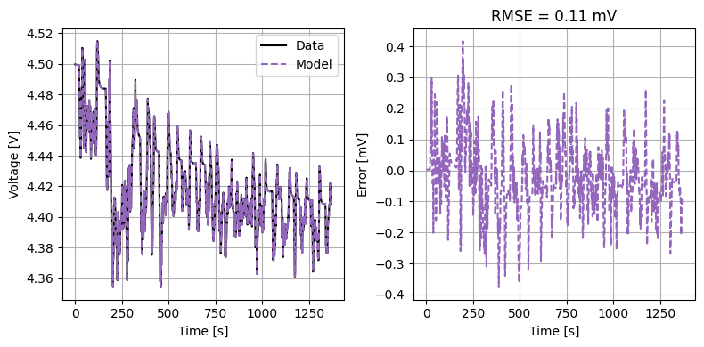
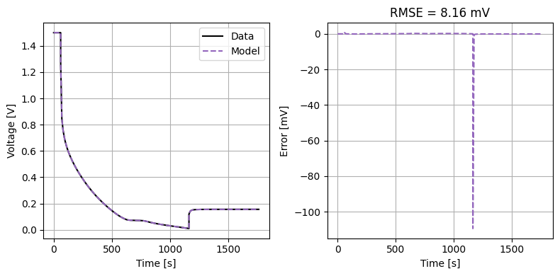
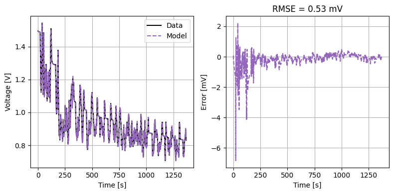
We can also run some validation experiments against the true parameters used to generate the synthetic data. We set up functions that run constant current and drive cycle experiments and plot the results

model = pybamm.lithium_ion.SPMe({"working electrode": "positive"})


def plot_constant_current(model, electrode, Crate=1):
    true_parameter_values = pybamm.ParameterValues(half_cell(electrode))
    constant_current(
        model,
        true_parameter_values,
        fitted_parameter_values[electrode],
        Crate=Crate,
        half_cell=True,
    )


def plot_drive_cycle(model, electrode, peak_current=None):
    true_parameter_values = pybamm.ParameterValues(half_cell(electrode))
    peak_current = peak_current or true_parameter_values["Nominal cell capacity [A.h]"]
    drive_cycle(
        model,
        true_parameter_values,
        fitted_parameter_values[electrode],
        peak_current=peak_current,
        half_cell=True,
    )

plot_constant_current(model, "negative", Crate=1)

plot_drive_cycle(model, "negative")

plot_constant_current(model, "positive", Crate=1)

plot_drive_cycle(model, "positive")