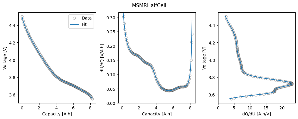
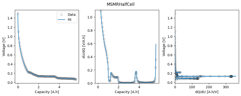
1. Half-cell OCP

In this example, we use the MSMR model to fit the half-cell OCPs, using the synthetic GITT data for each half-cell. The fitted parameters are saved to the “fitted_parameters” folder for use in later examples.

Before running this example, make sure to run the script true_parameters/generate_data.py to generate the synthetic data.

from pathlib import Path

import ionworkspipeline as iwp
import pandas as pd
import iwutil

We first set up our initial guesses for the parameters in each electrode. For the MSMR model, good initial guesses can be found using dVdQ analysis and/or by first using the iwp.optimizers.Interactive() optimizer, which allows users to interactively fit the model to the data in a Jupyter notebook.

def initial_guess(electrode):
    if electrode == "negative":
        ocp_msmr_param_init = {
            "U0_n_0": 0.08,
            "X_n_0": 0.30,
            "w_n_0": 0.1,
            "U0_n_1": 0.13,
            "X_n_1": 0.25,
            "w_n_1": 0.04,
            "U0_n_2": 0.15,
            "X_n_2": 0.15,
            "w_n_2": 0.9,
            "U0_n_3": 0.22,
            "X_n_3": 0.11,
            "w_n_3": 4.1,
            "U0_n_4": 0.22,
            "X_n_4": 0.03,
            "w_n_4": 0.05,
            "U0_n_5": 0.55,
            "X_n_5": 0.13,
            "w_n_5": 8.5,
        }
        voltage_limits = (0, 1.5)
    else:
        ocp_msmr_param_init = {
            "U0_p_0": 3.6,
            "X_p_0": 0.13,
            "w_p_0": 1,
            "U0_p_1": 3.7,
            "X_p_1": 0.32,
            "w_p_1": 1.4,
            "U0_p_2": 3.9,
            "X_p_2": 0.21,
            "w_p_2": 3.5,
            "U0_p_3": 4.2,
            "X_p_3": 0.33,
            "w_p_3": 5.5,
        }
        voltage_limits = (2.5, 5)
    ocp_msmr_param_init[f"Number of reactions in {electrode} electrode"] = int(
        len(ocp_msmr_param_init) // 3
    )
    return ocp_msmr_param_init, voltage_limits

Next we create a function to fit, plot and save the results for each half-cell.

The function first loads in and processes the data, then sets up the parameters to be fitted. In the MSMR model we fit the reaction potentials \(U_j\), the fractional site occupancies \(X_j\) (or, equivalently, the fractional capacities \(Q_j\)), and the parameters \(\omega_j\) that describe the level of disorder of the reaction represented by \(j\). We can also fit the electrode capacity and lower excess capacity. Initial values and bounds are set when creating the iwp.Parameter objects.

Next we set up the MSMR objective and datafit, and create a pipeline that first fits the MSMR model parameters to the data, and then saves the fitted stoichiometry-voltage values which can subsequently be used to create a parameter set for a lithium-ion model.

Finally, we fit the model to the data and plot the results. The fitted parameters are saved to the “fitted_parameters” folder for use in later examples.

def fit_plot_save(electrode):
    Electrode = electrode.capitalize()
    # Load data
    gitt_data = pd.read_csv(
        Path("synthetic_data") / f"half_cell_{electrode}_electrode" / "gitt.csv"
    )
    # Extract relaxed voltages from GITT to get OCP data
    ocp_data = iwp.data_fits.preprocess.pulse_data_to_ocp(gitt_data)

    # Initialize Parameter objects to be fitted
    Q_use = ocp_data["Capacity [A.h]"].max()
    ocp_msmr_param_init, voltage_limits = initial_guess(electrode)
    # helper function add U0_j, Q_j and w_j Parameters
    ocp_msmr_params = iwp.objectives.get_msmr_params_for_fit(
        ocp_msmr_param_init, electrode, Q_use, species_format="Qj"
    )
    # and the lower excess capacity
    # Add additional parameters
    ocp_msmr_params.update(
        {
            f"{Electrode} electrode lower excess capacity [A.h]": (
                iwp.Parameter(
                    "Q_lowex", initial_value=0.01 * Q_use, bounds=(0, 0.2 * Q_use)
                )
            ),
        }
    )

    # Set up objective and data fit
    # we can set dUdq_cutoff to ignore extrema in the dUdq curve
    dUdQ_cutoff = iwp.data_fits.util.calculate_dUdQ_cutoff(ocp_data)
    objective = iwp.objectives.MSMRHalfCell(
        electrode,
        ocp_data,
        options={
            "dUdQ cutoff": dUdQ_cutoff,
        },
    )
    ocp_msmr = iwp.DataFit(objective, parameters=ocp_msmr_params)

    # Run the fit at the given temperature
    known_params = {"Ambient temperature [K]": 298.15}
    params_fit = ocp_msmr.run(known_params)

    # Plot results
    ocp_msmr.plot_fit_results()

    # Save the scalar parameters
    params_to_save = {k: v for k, v in params_fit.items() if k in ocp_msmr_param_init}
    Q_total = params_fit[f"{Electrode} electrode capacity [A.h]"]
    params_to_save.update(
        {
            f"Half-cell {electrode} electrode capacity [A.h]": Q_total,
        }
    )
    iwutil.save.json(
        params_to_save, Path("fitted_parameters") / f"{electrode}_electrode_ocp.json"
    )

    # Save the stoichiometry-voltage values
    df = iwp.data_fits.util.generate_msmr_ocp_data(
        electrode,
        voltage_limits,
        {**params_fit, **known_params},
    )

    iwutil.save.csv(df, f"fitted_parameters/{electrode}_electrode_ocp.csv")

    return params_fit

Then we run the fit for each electrode

for electrode in ["positive", "negative"]:
    print(electrode)
    params_fit = fit_plot_save(electrode)

positive

negative

/home/docs/checkouts/readthedocs.org/user_builds/ionworks-ionworkspipeline/envs/v0.3.6/lib/python3.11/site-packages/pybamm/expression_tree/functions.py:152: RuntimeWarning: overflow encountered in exp
  return self.function(*evaluated_children)