Fitting Arrhenius relationships to data

This example shows how to fit Arrhenius relationships to data using the ArrheniusLogLinear class.

We plan on adding more thermal functions in the future, so keep an eye out for updates!

import ionworkspipeline as iwp
import matplotlib.pyplot as plt
import pybamm
import pandas as pd
import numpy as np

/home/docs/checkouts/readthedocs.org/user_builds/ionworks-ionworkspipeline/envs/v0.8.2/lib/python3.12/site-packages/pybtex/plugin/__init__.py:26: UserWarning: pkg_resources is deprecated as an API. See https://setuptools.pypa.io/en/latest/pkg_resources.html. The pkg_resources package is slated for removal as early as 2025-11-30. Refrain from using this package or pin to Setuptools<81.
  import pkg_resources

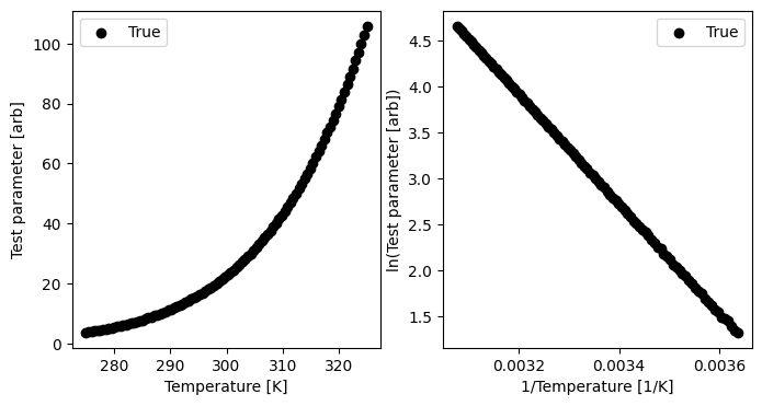
Begin by generating some synthetic data.

We will show this with a test parameter with units [arb], but this could be any parameter. The units are used to process the results. We add a bit of noise to the data to make it interesting.

R = pybamm.constants.R.value
T = np.linspace(275, 325, 100)
Ea_true = 50000.0
A_true = 20.0
T_ref = 298.15

param_name = "Test parameter [arb]"

# Set seed for reproducibility
np.random.seed(0)
param_val = A_true * np.exp(
    -Ea_true / (R * T) + Ea_true / (R * T_ref)
) + np.random.normal(0, 5e-2, len(T))

fig, ax = plt.subplots(1, 2, figsize=(8, 4))
ax[0].scatter(T, param_val, label="True", color="black")
ax[1].scatter(1 / T, np.log(param_val), label="True", color="black")
ax[0].set_xlabel("Temperature [K]")
ax[0].set_ylabel(param_name)
ax[1].set_xlabel("1/Temperature [1/K]")
ax[1].set_ylabel("ln(" + param_name + ")")
ax[0].legend()
ax[1].legend()

<matplotlib.legend.Legend at 0x768c59b5e990>

Now, we can fit the Arrhenius relationship using the ArrheniusLogLinear class provided by ionworkspipeline. The class takes as input a pandas DataFrame with the temperature and the parameter of interest. The reference temperature is optional, and if not provided, no reference temperature is used in the fit. Running the fit returns a dict with the activation energy, the pre-exponential factor (A), the reference temperature if provided, and a function for the parameter as a function of temperature.

arrh_fitter = iwp.calculations.ArrheniusLogLinear(
    pd.DataFrame({"Temperature [K]": T, param_name: param_val}),
    reference_temperature=T_ref,
    include_func=True,
)
param_values = arrh_fitter.run()
print(
    "Pre-exponential factor for test parameter [arb]:",
    param_values["Pre-exponential factor for test parameter [arb]"],
)
print("True pre-exponential factor for test parameter [arb]:", A_true)
print(
    "Activation energy for test parameter [J.mol-1]:",
    param_values["Activation energy for test parameter [J.mol-1]"],
)
print("True activation energy for test parameter [J.mol-1]:", Ea_true)
print("\n")
print("Full dict of results:")
print(param_values)


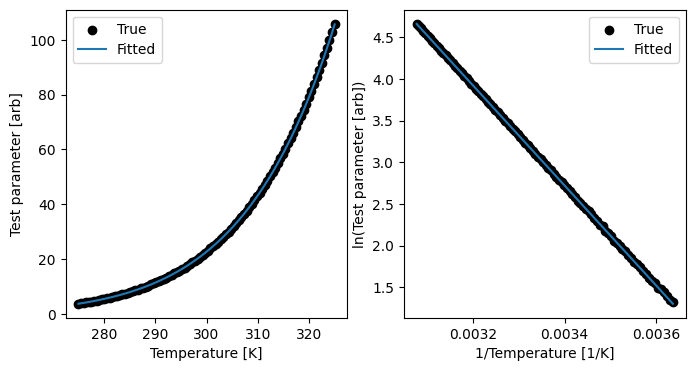
ax[0].plot(T, param_values["Test parameter [arb]"](T), label="Fitted")
ax[1].plot(
    1 / T, [np.log(param_values["Test parameter [arb]"](t)) for t in T], label="Fitted"
)
ax[0].legend()
ax[1].legend()
fig

Pre-exponential factor for test parameter [arb]: 20.023577251710947
True pre-exponential factor for test parameter [arb]: 20.0
Activation energy for test parameter [J.mol-1]: 49900.62291042594
True activation energy for test parameter [J.mol-1]: 50000.0


Full dict of results:
{'Activation energy for test parameter [J.mol-1]': 49900.62291042594, 'Reference temperature for test parameter [K]': 298.15, 'Pre-exponential factor for test parameter [arb]': 20.023577251710947, 'Test parameter [arb]': <function ArrheniusLogLinear.run.<locals>.<lambda> at 0x768c59b76340>}

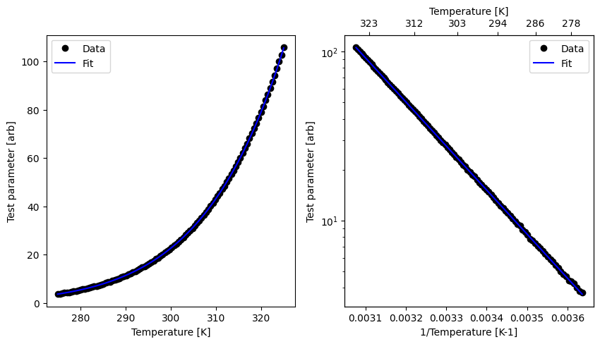
We also provide a plot_arrhenius method that plots the Arrhenius relationship once the calculation has been run.

fig, ax = arrh_fitter.plot_arrhenius()