Initial Guesses
In this example, we demonstrate how to
randomly generate initial guesses
run a pre-screening step to filter the top multistarts
optimize the best initial guess candidates
We begin by generating some synthetic data from a battery model.
import pybamm
import ionworkspipeline as iwp
import numpy as np
import pandas as pd
import matplotlib.pyplot as plt

# Load the model and parameter values
model = pybamm.lithium_ion.SPM()
parameter_values = iwp.ParameterValues("Chen2020")
parameter_values.update(
    {
        "Negative electrode active material volume fraction": 0.75,
        "Positive electrode active material volume fraction": 0.665,
    }
)

# Generate the data
t = np.arange(0, 900, 3)
sim = iwp.Simulation(
    model, parameter_values=parameter_values, t_eval=[0, 900], t_interp=t
)
sol = sim.solve()
data = pd.DataFrame(
    {x: sim.solution[x](t) for x in ["Time [s]", "Current [A]", "Voltage [V]"]}
)
# add noise to the data
sigma = 0.001
data["Voltage [V]"] += np.random.normal(0, sigma, len(data))
/home/docs/checkouts/readthedocs.org/user_builds/ionworks-ionworkspipeline/envs/v0.8.2/lib/python3.12/site-packages/pybtex/plugin/__init__.py:26: UserWarning: pkg_resources is deprecated as an API. See https://setuptools.pypa.io/en/latest/pkg_resources.html. The pkg_resources package is slated for removal as early as 2025-11-30. Refrain from using this package or pin to Setuptools<81.
  import pkg_resources
Next, we define the parameters to fit and their bounds. We apply a Log10 transform to the parameters, which optimizes and randomly generates the parameters on a logarithmic basis.
parameters = {
    "Negative electrode active material volume fraction": iwp.transforms.Log10(
        iwp.Parameter(
            "Negative electrode active material volume fraction",
            bounds=(0.55, 1),
        )
    ),
    "Positive electrode active material volume fraction": iwp.transforms.Log10(
        iwp.Parameter(
            "Positive electrode active material volume fraction",
            bounds=(0.45, 1),
        )
    ),
}
We set up the objective function, which in this case is the current driven objective. This takes the time vs current data and runs the model, comparing the model’s predictions for the voltage with the experimental data.
objective = iwp.objectives.CurrentDriven(data, options={"model": model})
Then, we set up the DataFit object, which takes the objective function, the parameters to fit, and the optimizer as inputs. Here we use the PointEstimate optimizer, which evaluates the cost function for a single set of parameters. We sample 300 randomly chosen parameters using the multistarts keyword argument.
optimizer = iwp.optimizers.PointEstimate()
data_fit = iwp.DataFit(
    objective,
    parameters=parameters,
    optimizer=optimizer,
    multistarts=200,
    options={"seed": 0},
)
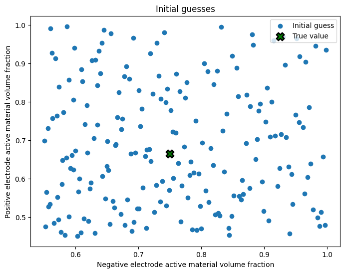
Before running the DataFit, we can visualize all the initial guess candidates using a scatterplot.
names = list(parameters.keys())

# Collect the initial guesses for each parameter
initial_guesses = data_fit.initial_guesses
initial_guess_arrays = {k: [ig[k] for ig in initial_guesses] for k in names}

fig, ax = plt.subplots(figsize=(8, 6))
ax.scatter(
    initial_guess_arrays[names[0]],
    initial_guess_arrays[names[1]],
    label="Initial guess",
)

# Add marker for the true parameter values
ax.scatter(
    parameter_values[names[0]],
    parameter_values[names[1]],
    c="green",
    s=120,
    marker="X",
    edgecolors="black",
    linewidth=2,
    label="True value",
)

ax.legend(loc="upper right")
ax.set_xlabel(names[0])
ax.set_ylabel(names[1])
ax.set_title("Initial guesses")
plt.show()
Next, we run the data fit, passing the parameters that are not being fit as a dictionary.
params_for_pipeline = {k: v for k, v in parameter_values.items() if k not in parameters}
results = data_fit.run(params_for_pipeline)
for k, v in results.items():
    print(f"{k}: {parameter_values[k]:.3e} (true) {v:.3e} (fit)")
/home/docs/checkouts/readthedocs.org/user_builds/ionworks-ionworkspipeline/envs/v0.8.2/lib/python3.12/site-packages/pybtex/plugin/__init__.py:26: UserWarning: pkg_resources is deprecated as an API. See https://setuptools.pypa.io/en/latest/pkg_resources.html. The pkg_resources package is slated for removal as early as 2025-11-30. Refrain from using this package or pin to Setuptools<81.
  import pkg_resources
Negative electrode active material volume fraction: 7.500e-01 (true) 7.135e-01 (fit)
Positive electrode active material volume fraction: 6.650e-01 (true) 6.758e-01 (fit)
Next, we plot the results and the trace of the cost function and parameter values.
out = data_fit.plot_fit_results()

out["CurrentDriven"][0][0].suptitle(f"Initial guesses, min cost: {results.costs:.5e}")
Text(0.5, 0.98, 'Initial guesses, min cost: 4.68993e-04')
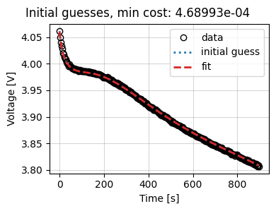
In the above plot, the initial guess and the fit lines fall on top of one another since no optimization is performed. The best-performing initial guess does a decent job of fitting the data, but there is still room for improvement.
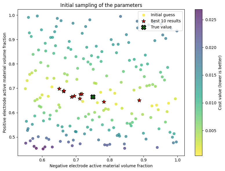
Let’s revisit the initial guess scatterplot where markers are colored by their cost function (lighter colors are better). The top 10 initial guesses are highlighted with a star.
# Number of best results to highlight
keep_best = 10

# Get the best results based on lowest cost
best_results = results.best_results(keep_best)

# Get parameter names
names = list(parameters.keys())

# Extract all initial guesses and their costs
initial_guesses = results.children
initial_guess_arrays = {k: [ig[k] for ig in initial_guesses] for k in names}
costs = [r.costs.min() for r in results.children]

# Convert costs to numpy array for easier manipulation
costs_array = np.array(costs)

# Sort results by cost (ascending order)
sort_indices = np.argsort(costs_array)
x_sorted = np.array(initial_guess_arrays[names[0]])[sort_indices]
y_sorted = np.array(initial_guess_arrays[names[1]])[sort_indices]
costs_sorted = costs_array[sort_indices]

# Create figure showing all results colored by cost
fig, ax = plt.subplots(figsize=(8, 6))

# Plot all points with color indicating cost value
scatter = ax.scatter(
    x_sorted,
    y_sorted,
    c=costs_sorted,
    cmap="viridis_r",  # Reversed colormap so lower costs are darker
    alpha=0.7,
    label="Initial guess",
)

# Highlight the best results with star markers
ax.scatter(
    x_sorted[:keep_best],
    y_sorted[:keep_best],
    c="red",
    s=100,
    marker="*",
    edgecolors="black",
    label=f"Best {keep_best} results",
)

# Add marker for the true parameter values
ax.scatter(
    parameter_values[names[0]],
    parameter_values[names[1]],
    c="green",
    s=120,
    marker="X",
    edgecolors="black",
    linewidth=2,
    label="True value",
)

# Add colorbar and labels
plt.colorbar(scatter, label="Cost value (lower is better)")
ax.set_xlabel(names[0])
ax.set_ylabel(names[1])
ax.legend(loc="upper right")
ax.set_title("Initial sampling of the parameters")
plt.tight_layout()
plt.show()
After the pre-screening step, we create another DataFit which uses the top 10 best-performing initial guesses in a full optimization run.
optimizer = iwp.optimizers.ScipyMinimize(method="Nelder-Mead")

data_fit_refined = iwp.DataFit(
    objective,
    parameters=parameters,
    initial_guesses=best_results,
)

results_refined = data_fit_refined.run(params_for_pipeline)
for k, v in results_refined.items():
    print(f"{k}: {parameter_values[k]:.3e} (true) {v:.3e} (fit)")
Negative electrode active material volume fraction: 7.500e-01 (true) 7.480e-01 (fit)
Positive electrode active material volume fraction: 6.650e-01 (true) 6.653e-01 (fit)
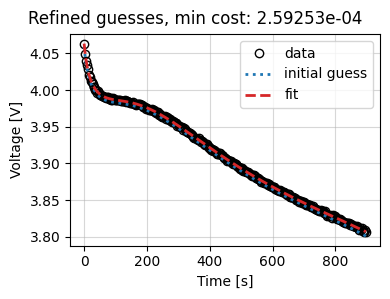
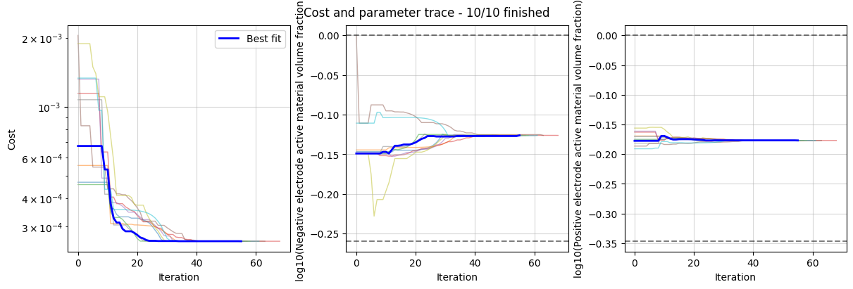
Finally, we plot the refined results and the trace of the cost function and parameter values.
out_refined = data_fit_refined.plot_fit_results()

out_refined["CurrentDriven"][0][0].suptitle(
    f"Refined guesses, min cost: {results_refined.costs.min():.5e}"
)

_ = data_fit_refined.plot_trace()