Half-cell OCP fitting

In this example, we show how to fit the half-cell Open-Circuit Potential to pseudo-OCP data. Our recommended workflow for fitting OCPs is to first fit the MSMR model to the data and then create an interpolant to find a function \(U(x)\), where \(x\) is the stoichiometry. For comparison, we also show how to fit a function \(U(x)\) directly to pseudo-OCP data.

import ionworkspipeline as iwp
import numpy as np
import pandas as pd
import pybamm
import matplotlib.pyplot as plt
from scipy.signal import savgol_filter

/home/docs/checkouts/readthedocs.org/user_builds/ionworks-ionworkspipeline/envs/v0.8.2/lib/python3.12/site-packages/pybtex/plugin/__init__.py:26: UserWarning: pkg_resources is deprecated as an API. See https://setuptools.pypa.io/en/latest/pkg_resources.html. The pkg_resources package is slated for removal as early as 2025-11-30. Refrain from using this package or pin to Setuptools<81.
  import pkg_resources

Pre-process and visualize the data

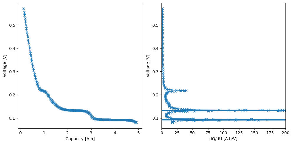
First, we load and pre-process the data.

# Load data
raw_ocp_data = pd.read_csv("anode_ocp_delithiation.csv", comment="#")
q = raw_ocp_data["Capacity [A.h]"].values
U = raw_ocp_data["Voltage [V]"].values

# Smooth
q_smoothed = savgol_filter(q, window_length=11, polyorder=1)
U_smoothed = savgol_filter(U, window_length=11, polyorder=1)
dQdU_smoothed = -np.gradient(q_smoothed, U_smoothed)

# Store in a dataframe
ocp_data = pd.DataFrame({"Capacity [A.h]": q_smoothed, "Voltage [V]": U_smoothed})
ocp_data = iwp.data_fits.preprocess.sort_capacity_and_ocp(ocp_data)
# Maximum capacity, will be used later as an initial guess for the electrode capacity
Q_max_data = ocp_data["Capacity [A.h]"].max()

# Plot
_, ax = plt.subplots(1, 2, figsize=(10, 5))
ax[0].plot(q_smoothed, U_smoothed, "-x")
ax[0].set_xlabel("Capacity [A.h]")
ax[0].set_ylabel("Voltage [V]")
ax[1].plot(dQdU_smoothed, U_smoothed, "-x")
ax[1].set_xlabel("dQ/dU [A.h/V]")
ax[1].set_ylabel("Voltage [V]")
ax[1].set_xlim(0, 200)
plt.tight_layout()

/home/docs/checkouts/readthedocs.org/user_builds/ionworks-ionworkspipeline/envs/v0.8.2/lib/python3.12/site-packages/numpy/lib/function_base.py:1242: RuntimeWarning: divide by zero encountered in divide
  a = -(dx2)/(dx1 * (dx1 + dx2))
/home/docs/checkouts/readthedocs.org/user_builds/ionworks-ionworkspipeline/envs/v0.8.2/lib/python3.12/site-packages/numpy/lib/function_base.py:1243: RuntimeWarning: divide by zero encountered in divide
  b = (dx2 - dx1) / (dx1 * dx2)
/home/docs/checkouts/readthedocs.org/user_builds/ionworks-ionworkspipeline/envs/v0.8.2/lib/python3.12/site-packages/numpy/lib/function_base.py:1244: RuntimeWarning: divide by zero encountered in divide
  c = dx1 / (dx2 * (dx1 + dx2))
/home/docs/checkouts/readthedocs.org/user_builds/ionworks-ionworkspipeline/envs/v0.8.2/lib/python3.12/site-packages/numpy/lib/function_base.py:1250: RuntimeWarning: invalid value encountered in add
  out[tuple(slice1)] = a * f[tuple(slice2)] + b * f[tuple(slice3)] + c * f[tuple(slice4)]

Fit the MSMR model to data

We begin by getting literature values for the MSMR parameters from the ionworkspipeline library

lib = iwp.Library()
gr = lib["Graphite - Verbrugge 2017"]
gr_params = gr.parameter_values

This gives us initial guesses for the MSMR species parameters (\(X_j\), \(U^0_j\), and \(w_j\)). We also need estimates for the total electrode capacity and lower excess capacity. We can use the helper function get_initial_capacity_and_lower_excess_capacity to estimate these from the species parameters and data

gr_params.update(
    iwp.data_fits.objectives.get_initial_capacity_and_lower_excess_capacity(
        gr_params, "negative", ocp_data
    )
)

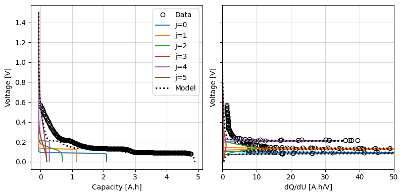
We can plot these against the data and, if required, manually adjust them to get a better starting point. For this example, let’s keep the Graphite parameters as our initial guess.

fig, ax = iwp.objectives.plot_each_species_msmr(
    ocp_data, gr_params, "negative", voltage_limits=(0, 1.5)
)
_ = ax[1].set_xlim(0, 50)

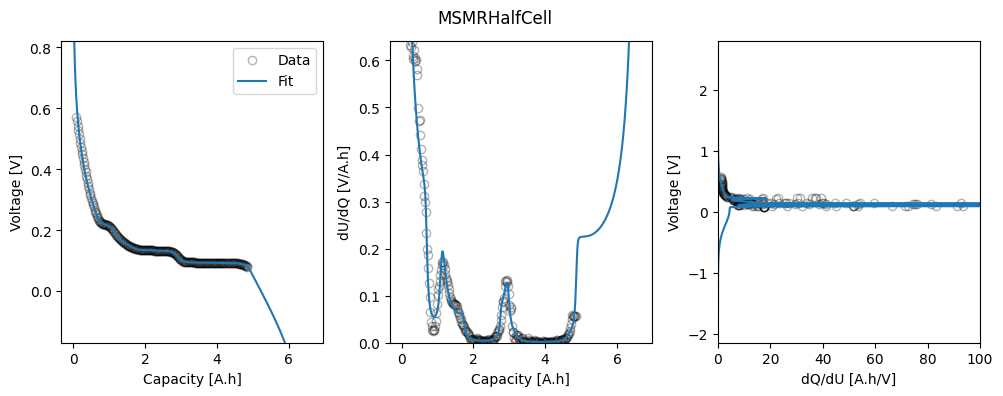
Now we can set up the objective and parameters to fit, run the data fit and plot the results.

# Loop over the initial guesses and set up the parameters to fit with appropriate bounds
parameters_to_fit = {}
for k, v in iwp.parameter_values.scalarize_dict(gr_params).items():
    if "host site occupancy fraction" in k:
        bounds = (0, 1)
    elif "host site standard potential" in k:
        bounds = (max(0, v - 0.5), v + 0.5)
    elif "host site ideality factor" in k:
        bounds = (1e-2, 100)
    elif "lower excess" in k:
        bounds = (0, 0.1 * Q_max_data)
    elif "capacity" in k:
        bounds = (Q_max_data, 1.5 * Q_max_data)
    else:
        continue
    parameters_to_fit[k] = iwp.Parameter(k, initial_value=v, bounds=bounds)

# Calculate dUdQ cutoff to prevent overfitting to extreme dUdQ values
dUdq_cutoff = iwp.data_fits.util.calculate_dUdQ_cutoff(ocp_data)

# Set up model, objective and fit
model = iwp.data_fits.models.MSMRHalfCellModel(
    "negative", options={"species format": "Xj"}
)
objective = iwp.data_fits.objectives.MSMRHalfCell(
    ocp_data, options={"model": model, "dUdQ cutoff": dUdq_cutoff}
)
ocp_msmr = iwp.DataFit(
    objective,
    parameters=parameters_to_fit,
)

# Run the fit
results = ocp_msmr.run({"Ambient temperature [K]": 298.15})

# Plot results
fig_ax = ocp_msmr.plot_fit_results()
axes = fig_ax["MSMRHalfCell"][0][1]
_ = axes[2].set_xlim(0, 100)

Lastly, we can look at the fitted parameters.

ocp_msmr.results

Result(
  Negative electrode host site ideality factor: [0.019526510055650457, 0....
  Negative electrode host site standard potential [V]: [0.092301148834443...
  Negative electrode host site occupancy fraction: [0.21916745240179422, ...
  Negative electrode capacity [A.h]: 6.63447
  Negative electrode lower excess capacity [A.h]: 0.0866398
)

We can access tabulated capacity vs OCP data from the MSMR callback

outputs = results.callbacks["MSMRHalfCell"].callbacks[0].fit_results_["outputs"]
q = outputs["Capacity [A.h]"]
U = outputs["Voltage [V]"]
ocp_fit_data = pd.DataFrame({"Capacity [A.h]": q, "Voltage [V]": U})
ocp_fit_data.head()

	Capacity [A.h]	Voltage [V]
0	0.036630	0.570425
1	0.046742	0.556259
2	0.057644	0.542092
3	0.069388	0.527926
4	0.082033	0.513760

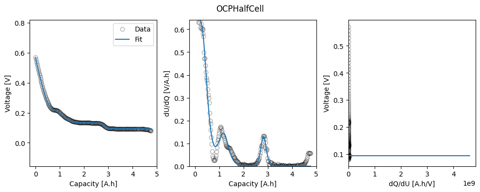
Fit OCP as a function of stoichiometry

Now, we directly fit a function \(U(x)\) to the pseudo-OCP data.

First, we define the function and initial guesses for the parameters.

def U_half_cell(theta):
    u00 = pybamm.Parameter("u00_pos")
    u10 = pybamm.Parameter("u10_pos")
    u11 = pybamm.Parameter("u11_pos")
    u20 = pybamm.Parameter("u20_pos")
    u21 = pybamm.Parameter("u21_pos")
    u22 = pybamm.Parameter("u22_pos")
    u30 = pybamm.Parameter("u30_pos")
    u31 = pybamm.Parameter("u31_pos")
    u32 = pybamm.Parameter("u32_pos")
    u40 = pybamm.Parameter("u40_pos")
    u41 = pybamm.Parameter("u41_pos")
    u42 = pybamm.Parameter("u42_pos")

    u_eq = (
        u00
        + u10 * pybamm.exp(-u11 * theta)
        + u20 * pybamm.tanh(u21 * (theta - u22))
        + u30 * pybamm.tanh(u31 * (theta - u32))
        + u40 * pybamm.tanh(u41 * (theta - u42))
    )

    return u_eq


ocp_param_init = {
    "u00_pos": 0.2,
    "u10_pos": 2,
    "u11_pos": 30,
    "u20_pos": -0.1,
    "u21_pos": 30,
    "u22_pos": 0.1,
    "u30_pos": -0.1,
    "u31_pos": 30,
    "u32_pos": 0.3,
    "u40_pos": -0.1,
    "u41_pos": 30,
    "u42_pos": 0.6,
}

Then we set up our DataFit object and fit the data.

# Set up Parameter objects to fit
ocp_params = {k: iwp.Parameter(k, initial_value=v) for k, v in ocp_param_init.items()}
# Add the functional form of the OCP
ocp_params = {"Positive electrode OCP [V]": U_half_cell, **ocp_params}

# Use the experimental capacity to map between capacity in the experiment and the
# stoichiometry. In practice we would calculate the capacity from other means,
# (e.g. electrode loading) or use the MSMR model to fit the electrode capacity.
known_parameter_values = {"Positive electrode capacity [A.h]": Q_max_data}

# Set up objective and fit
objective = iwp.objectives.OCPHalfCell(
    "positive",
    ocp_data,
)
ocp = iwp.DataFit(objective, parameters=ocp_params)

# Fit
params_fit_ocp = ocp.run(known_parameter_values)

# Plot
_ = ocp.plot_fit_results()

Then, we look at the fitted parameters.

params_fit_ocp

Result(
  Positive electrode OCP [V]: <function U_half_cell at 0x795bb01c60c0>
  u00_pos: 0.26766
  u10_pos: 0.148291
  u11_pos: 21.9377
  u20_pos: -0.115899
  u21_pos: 17.9201
  u22_pos: 0.0648092
  u30_pos: -0.0381474
  u31_pos: 17.4306
  u32_pos: 0.246712
  u40_pos: -0.0194789
  u41_pos: 32.1578
  u42_pos: 0.593834
)