EIS fiting

In this example we show how to fit parameters using EIS data. This objective uses package pybammeis to simulate the model response in the frequency domain.

import pybammeis
import pybamm
import pandas as pd
import ionworkspipeline as iwp
import numpy as np

Generate data

We begin by generating synthetic EIS data for a Gr//SiOx half-cell. We will specify the reference exchange-current density and double-layer capacitance, and then simulate the impedance response for a range of frequencies.

# Load model (DFN with capacitance)
model = pybamm.lithium_ion.DFN(
    options={"working electrode": "positive", "surface form": "differential"}
)

# Load parameters
parameter_values = pybamm.ParameterValues("OKane2022_graphite_SiOx_halfcell")


def j0(c_e, c_s_surf, c_s_max, T):
    j0_ref = pybamm.Parameter(
        "Positive electrode reference exchange-current density [A.m-2]"
    )
    c_e_init = pybamm.Parameter("Initial concentration in electrolyte [mol.m-3]")

    return (
        j0_ref
        * (c_e / c_e_init) ** 0.5
        * (c_s_surf / c_s_max) ** 0.5
        * (1 - c_s_surf / c_s_max) ** 0.5
    )


parameter_values.update(
    {
        "Positive electrode reference exchange-current density [A.m-2]": 2,
        "Positive electrode exchange-current density [A.m-2]": j0,
        "Positive electrode double-layer capacity [F.m-2]": 0.3,
    },
    check_already_exists=False,
)

# Create simulation
eis_sim = pybammeis.EISSimulation(model, parameter_values=parameter_values)

# Choose frequencies and calculate impedance
frequencies = np.logspace(-4, 4, 30)
sol = eis_sim.solve(frequencies)

# Store data as arrays of real and complex impedance
Z_Re = sol.real
Z_Im = sol.imag
data = pd.DataFrame(
    {"Frequency [Hz]": frequencies, "Z_Re [Ohm]": Z_Re, "Z_Im [Ohm]": Z_Im}
)

# Generate a Nyquist plot
eis_sim.nyquist_plot()

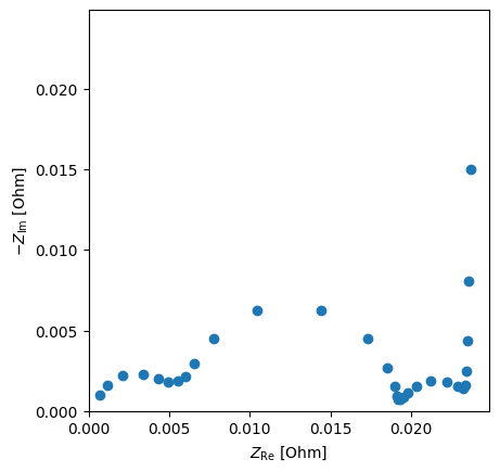
<Axes: xlabel='$Z_\\mathrm{Re}$ [Ohm]', ylabel='$-Z_\\mathrm{Im}$ [Ohm]'>

Fit parameters

We first set up the EIS objective. We pass in the data, model and frequency range.

objective = iwp.objectives.EIS(data, options={"model": model})

We can then specify which parameters need to be fitted (with initial guesses and bounds), which parameters are known, and pass this to the standard DataFit class to fit the unknown parameters

parameters = {
    "Positive electrode reference exchange-current density [A.m-2]": iwp.Parameter(
        "j0_p_ref", initial_value=1, bounds=(0.1, 10)
    ),
    "Positive electrode double-layer capacity [F.m-2]": iwp.Parameter(
        "C_dl_p", initial_value=0.1, bounds=(0.01, 1)
    ),
}
known_parameters = {k: v for k, v in parameter_values.items() if k not in parameters}

data_fit = iwp.DataFit(objective, parameters=parameters)

Next we run the fit and take a look at the results.

fitted_parameters = data_fit.run(known_parameters)
for name, p_fit in fitted_parameters.items():
    print(f"{name}: {p_fit} (fit) {parameter_values[name]} (true)")

Positive electrode reference exchange-current density [A.m-2]: 1.9999996109496305 (fit) 2 (true)
Positive electrode double-layer capacity [F.m-2]: 0.29999995719633366 (fit) 0.3 (true)

%load_ext autoreload
%autoreload 2

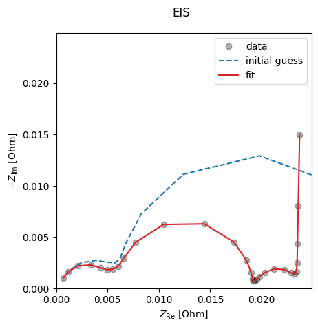
We can also plot the results

data_fit.plot_fit_results()

{'EIS': [(<Figure size 640x480 with 1 Axes>,
   <Axes: xlabel='$Z_\\mathrm{Re}$ [Ohm]', ylabel='$-Z_\\mathrm{Im}$ [Ohm]'>)]}

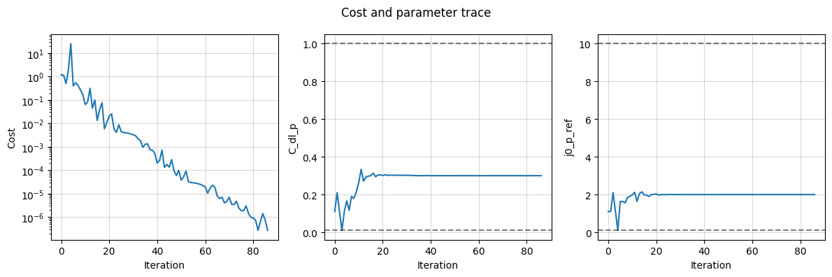
and the trace of the cost and the parameter values to see how the fit progressed

data_fit.plot_trace()

(<Figure size 1200x400 with 3 Axes>,
 array([<Axes: xlabel='Iteration', ylabel='Cost'>,
        <Axes: xlabel='Iteration', ylabel='C_dl_p'>,
        <Axes: xlabel='Iteration', ylabel='j0_p_ref'>], dtype=object))