Half-cell OCP fitting

In this example, we show how to fit the half-cell Open-Circuit Potential to pseudo-OCP data. Our recommended workflow for fitting OCPs is to first fit the MSMR model to the data and then create an interpolant to find a function \(U(x)\), where \(x\) is the stoichiometry. For comparison, we also show how to fit a function \(U(x)\) directly to pseudo-OCP data.

import ionworkspipeline as iwp
import numpy as np
import pandas as pd
import pybamm
import matplotlib.pyplot as plt
from scipy.signal import savgol_filter

Pre-process and visualize the data

First we load and pre-process the data

# Load data
raw_ocp_data = pd.read_csv("anode_ocp_delithiation.csv", comment="#")
q = raw_ocp_data["Capacity [A.h]"].values
U = raw_ocp_data["Voltage [V]"].values

# Smooth
q_smoothed = savgol_filter(q, window_length=11, polyorder=1)
U_smoothed = savgol_filter(U, window_length=11, polyorder=1)
dQdU_smoothed = -np.gradient(q_smoothed, U_smoothed)

# Store in a dataframe
ocp_data = pd.DataFrame({"Capacity [A.h]": q_smoothed, "Voltage [V]": U_smoothed})
ocp_data = iwp.data_fits.preprocess.sort_capacity_and_ocp(ocp_data)
# Maximum capacity, will be used later as an initial guess for the electrode capacity
Q_max_data = ocp_data["Capacity [A.h]"].max()

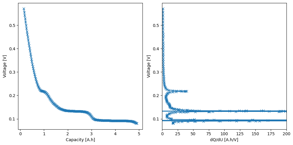
# Plot
_, ax = plt.subplots(1, 2, figsize=(10, 5))
ax[0].plot(q_smoothed, U_smoothed, "-x")
ax[0].set_xlabel("Capacity [A.h]")
ax[0].set_ylabel("Voltage [V]")
ax[1].plot(dQdU_smoothed, U_smoothed, "-x")
ax[1].set_xlabel("dQ/dU [A.h/V]")
ax[1].set_ylabel("Voltage [V]")
ax[1].set_xlim(0, 200)
plt.tight_layout()

/home/docs/checkouts/readthedocs.org/user_builds/ionworks-ionworkspipeline/envs/v0.3.6/lib/python3.11/site-packages/numpy/lib/function_base.py:1242: RuntimeWarning: divide by zero encountered in divide
  a = -(dx2)/(dx1 * (dx1 + dx2))
/home/docs/checkouts/readthedocs.org/user_builds/ionworks-ionworkspipeline/envs/v0.3.6/lib/python3.11/site-packages/numpy/lib/function_base.py:1243: RuntimeWarning: divide by zero encountered in divide
  b = (dx2 - dx1) / (dx1 * dx2)
/home/docs/checkouts/readthedocs.org/user_builds/ionworks-ionworkspipeline/envs/v0.3.6/lib/python3.11/site-packages/numpy/lib/function_base.py:1244: RuntimeWarning: divide by zero encountered in divide
  c = dx1 / (dx2 * (dx1 + dx2))
/home/docs/checkouts/readthedocs.org/user_builds/ionworks-ionworkspipeline/envs/v0.3.6/lib/python3.11/site-packages/numpy/lib/function_base.py:1250: RuntimeWarning: invalid value encountered in add
  out[tuple(slice1)] = a * f[tuple(slice2)] + b * f[tuple(slice3)] + c * f[tuple(slice4)]

Fit the MSMR model to data

We begin by setting up initial guesses for our MSMR parameters

# Initial guess of Graphite from Verbrugge et al 2017 J. Electrochem. Soc. 164 E3243
msmr_param_init = {
    "U0_p_0": 0.088,
    "X_p_0": 0.43,
    "w_p_0": 0.086,
    "U0_p_1": 0.13,
    "X_p_1": 0.24,
    "w_p_1": 0.080,
    "U0_p_2": 0.14,
    "X_p_2": 0.15,
    "w_p_2": 0.72,
    "U0_p_3": 0.17,
    "X_p_3": 0.055,
    "w_p_3": 2.5,
    "U0_p_4": 0.21,
    "X_p_4": 0.067,
    "w_p_4": 0.095,
    "U0_p_5": 0.36,
    "X_p_5": 0.055,
    "w_p_5": 6.0,
    "Number of reactions in positive electrode": 6,
    "Positive electrode lower excess capacity [A.h]": 0.0,
    "Positive electrode capacity [A.h]": Q_max_data,
    "Ambient temperature [K]": 298.15,
}

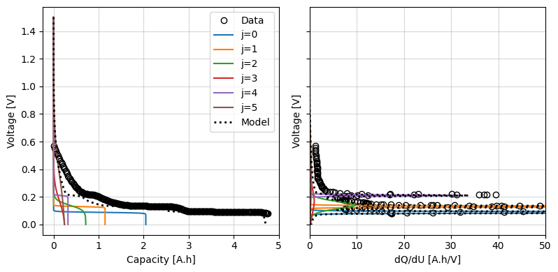
We can plot these against the data and, if required, manually adjust them to get a better starting point. For this example, let’s keep the Graphite parameters as our initial guess

fig, ax = iwp.objectives.plot_each_species_msmr(
    ocp_data, msmr_param_init, "positive", voltage_limits=(0, 1.5)
)
ax[1].set_xlim(0, 50)

(0.0, 50.0)

Now we can set up the objective and parameters to fit, run the data fit and plot the results

# Pass in the lithiation function, and fit the electrode capacity and lower excess
# capacity by making them Parameter objects
n_species = msmr_param_init["Number of reactions in positive electrode"]
theta_half_cell = iwp.objectives.get_theta_half_cell_msmr(n_species, "positive")
msmr_params = {
    "Positive electrode lithiation": theta_half_cell,
    "Ambient temperature [K]": 298.15,
    "Positive electrode capacity [A.h]": iwp.Parameter(
        "Q", initial_value=Q_max_data, bounds=(0.9 * Q_max_data, 1.2 * Q_max_data)
    ),
    "Positive electrode lower excess capacity [A.h]": (
        iwp.Parameter(
            "Q_lowex", initial_value=0.01 * Q_max_data, bounds=(0, 0.01 * Q_max_data)
        )
    ),
}
# Add Parameter objects for the MSMR parameters X_j, U0_j, and w_j
for k, v in msmr_param_init.items():
    if "X" in k:
        bounds = (0, 1)
    elif "U0_" in k:
        # allow a 500 mV variation either way
        bounds = (max(0, v - 0.5), v + 0.5)
    elif "w_" in k:
        bounds = (1e-2, 100)
    else:
        continue
    msmr_params[k] = iwp.Parameter(k, initial_value=v, bounds=bounds)

# Calculate dUdQ cutoff to prevent overfitting to extreme dUdQ values
dUdq_cutoff = iwp.data_fits.util.calculate_dUdQ_cutoff(ocp_data)

# Set up objective and fit
objective = iwp.objectives.MSMRHalfCell(
    "positive", ocp_data, options={"dUdQ cutoff": dUdq_cutoff}
)
ocp_msmr = iwp.DataFit(objective, parameters=msmr_params)

# Run the fit
params_fit_msmr = ocp_msmr.run({})

# Plot results
fig_ax = ocp_msmr.plot_fit_results()
axes = fig_ax["MSMRHalfCell"][0][1]
_ = axes[2].set_xlim(0, 100)

/home/docs/checkouts/readthedocs.org/user_builds/ionworks-ionworkspipeline/envs/v0.3.6/lib/python3.11/site-packages/pybamm/expression_tree/functions.py:152: RuntimeWarning: overflow encountered in exp
  return self.function(*evaluated_children)

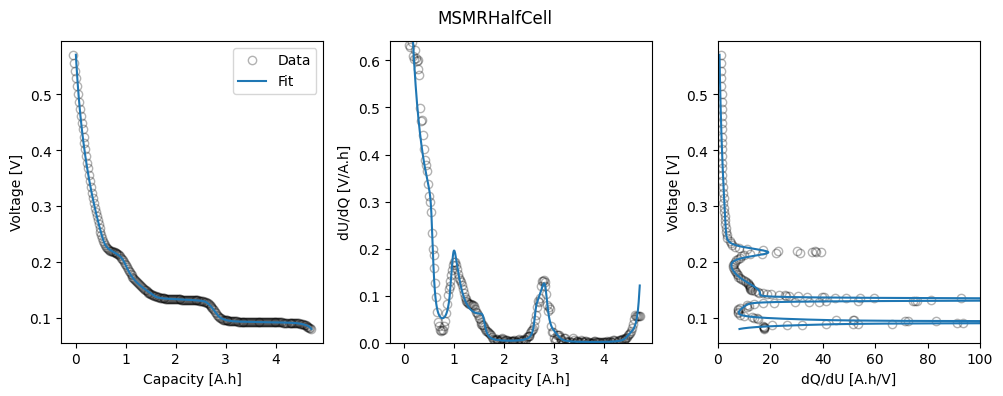
and look at the fitted parameters

params_fit_msmr

{'Positive electrode lithiation': functools.partial(<function _theta_half_cell at 0x7f14a8610f40>, 6, 'positive', 'Xj', None),
 'Ambient temperature [K]': 298.15,
 'Positive electrode capacity [A.h]': 5.192359137609005,
 'Positive electrode lower excess capacity [A.h]': 0.047630270342331985,
 'U0_p_0': 0.09230146500093617,
 'X_p_0': 0.21932912934996304,
 'w_p_0': 0.019189398402211705,
 'U0_p_1': 0.13287143432723472,
 'X_p_1': 0.17031108441704762,
 'w_p_1': 0.03971404823345671,
 'U0_p_2': 0.21720299707172705,
 'X_p_2': 0.054898616291004974,
 'w_p_2': 0.17809007204186386,
 'U0_p_3': 0.14432525106155114,
 'X_p_3': 0.11586723764717108,
 'w_p_3': 0.5004700827689491,
 'U0_p_4': 0.0921578213033519,
 'X_p_4': 0.11742016403402523,
 'w_p_4': 0.10983137135414951,
 'U0_p_5': 1.214931203008108e-07,
 'X_p_5': 0.663035453953011,
 'w_p_5': 6.352222770542614}

This MSMR fit can then be used to generate an interpolant for the OCP either manually or using the OCPMSMRInterpolant pipeline element

voltage_limits = (0, 1.5)
ocp_msmr_interpolant = iwp.calculations.OCPMSMRInterpolant("positive", voltage_limits)
params_fit_msmr_interpolant = ocp_msmr_interpolant.run(params_fit_msmr)

We can see in the returned parameter values that we have a “Positive electrode OCP [V]” function as well as the original data.

params_fit_msmr_interpolant

{'Positive electrode OCP [V]': <function ionworkspipeline.calculations.ocp_interpolant.OCPMSMRInterpolant.run.<locals>.U(sto)>,
 'Positive electrode OCP data [V]': array([[6.75985722e-05, 6.82232908e-05, 6.88537823e-05, ...,
         1.00629222e+00, 1.00781736e+00, 1.00934254e+00],
        [1.50000000e+00, 1.49849850e+00, 1.49699700e+00, ...,
         3.00300300e-03, 1.50150150e-03, 0.00000000e+00]])}

We can access the “data” generated from the MSMR function as follows:

theta_U = ocp_msmr_interpolant.fit_results_["interpolant"]
theta = theta_U[0]  # stoichiometry
U = theta_U[1]  # potential

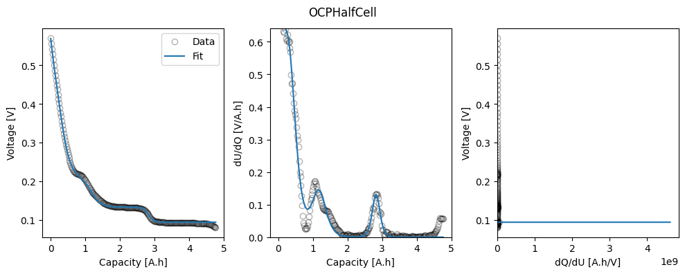
Fit OCP as a function of stoichiometry

Now we directly fit a function \(U(x)\) to the pseudo-OCP data.

First we define the function and initial guesses for the parameters.

def U_half_cell(theta):
    u00 = pybamm.Parameter("u00_pos")
    u10 = pybamm.Parameter("u10_pos")
    u11 = pybamm.Parameter("u11_pos")
    u20 = pybamm.Parameter("u20_pos")
    u21 = pybamm.Parameter("u21_pos")
    u22 = pybamm.Parameter("u22_pos")
    u30 = pybamm.Parameter("u30_pos")
    u31 = pybamm.Parameter("u31_pos")
    u32 = pybamm.Parameter("u32_pos")
    u40 = pybamm.Parameter("u40_pos")
    u41 = pybamm.Parameter("u41_pos")
    u42 = pybamm.Parameter("u42_pos")

    u_eq = (
        u00
        + u10 * pybamm.exp(-u11 * theta)
        + u20 * pybamm.tanh(u21 * (theta - u22))
        + u30 * pybamm.tanh(u31 * (theta - u32))
        + u40 * pybamm.tanh(u41 * (theta - u42))
    )

    return u_eq


ocp_param_init = {
    "u00_pos": 0.2,
    "u10_pos": 2,
    "u11_pos": 30,
    "u20_pos": -0.1,
    "u21_pos": 30,
    "u22_pos": 0.1,
    "u30_pos": -0.1,
    "u31_pos": 30,
    "u32_pos": 0.3,
    "u40_pos": -0.1,
    "u41_pos": 30,
    "u42_pos": 0.6,
}

Then we set up our DataFit object and fit the data

# Set up Parameter objects to fit
ocp_params = {k: iwp.Parameter(k, initial_value=v) for k, v in ocp_param_init.items()}
# Add the functional form of the OCP
ocp_params = {"Positive electrode OCP [V]": U_half_cell, **ocp_params}

# Use the experimental capacity to map between capacity in the experiment and the
# stoichiometry. In practice we would calculate the capacity from other means,
# (e.g. electrode loading) or use the MSMR model to fit the electrode capacity.
known_parameter_values = {"Positive electrode capacity [A.h]": Q_max_data}

# Set up objective and fit
objective = iwp.objectives.OCPHalfCell(
    "positive",
    ocp_data,
)
ocp = iwp.DataFit(objective, parameters=ocp_params)

# Fit
params_fit_ocp = ocp.run(known_parameter_values)

# Plot
_ = ocp.plot_fit_results()

and look at the fitted parameters

params_fit_ocp

{'Positive electrode OCP [V]': <function __main__.U_half_cell(theta)>,
 'u00_pos': 0.2676574400954305,
 'u10_pos': 0.1482804774849739,
 'u11_pos': 21.938773174842293,
 'u20_pos': -0.11590651680821173,
 'u21_pos': 17.919629397234793,
 'u22_pos': 0.06480833133627988,
 'u30_pos': -0.0381460004259179,
 'u31_pos': 17.431611556478156,
 'u32_pos': 0.24671015843772892,
 'u40_pos': -0.01947908929632694,
 'u41_pos': 32.15754846722795,
 'u42_pos': 0.5938341015563623}