Using callbacks in objectives

This notebook explains how to use a callback in an objective function. Potential use cases for this are:

• Plotting some outputs at each iteration of the optimization

• Saving internal variables to plot once the optimization is complete

Some objectives have “internal callbacks” which are not intended to be user facing. These are standard callbacks that can be used to plot the results of an optimization by using DataFit.plot_fit_results(). For user-facing callbacks, users should create their own callback objects and call them directly for plotting, as demonstrated in this notebook

Creating a custom callback

To implement a custom callback, we create a class that inherits from iwp.callbacks.Callback and calls some specific functions. See the documentation for iwp.callbacks.Callback for more information on the available functions and their expected inputs.

import ionworkspipeline as iwp
import matplotlib.pyplot as plt
import pybamm
import numpy as np
import pandas as pd

class MyCallback(iwp.callbacks.Callback):
    def __init__(self):
        super().__init__()
        # Implement our own iteration counter
        self.iter = 0

    def on_objective_build(self, logs):
        self.data_ = logs["data"]

    def on_run_iteration(self, logs):
        # Print some information at each iteration
        inputs = logs["inputs"]
        V_model = logs["outputs"]["Voltage [V]"]
        V_data = self.data_["Voltage [V]"]

        # calculate RMSE, note this is not necessarily the cost function used in the optimization
        rmse = np.sqrt(np.nanmean((V_model - V_data) ** 2))

        print(f"Iteration: {self.iter}, Inputs: {inputs}, RMSE: {rmse}")
        self.iter += 1

    def on_datafit_finish(self, logs):
        self.fit_results_ = logs

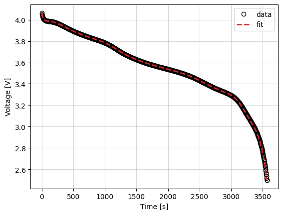
    def plot_fit_results(self):
        """
        Plot the fit results.
        """
        data = self.data_
        fit = self.fit_results_["outputs"]

        fit_results = {
            "data": (data["Time [s]"], data["Voltage [V]"]),
            "fit": (fit["Time [s]"], fit["Voltage [V]"]),
        }

        markers = {"data": "o", "fit": "--"}
        colors = {"data": "k", "fit": "tab:red"}
        fig, ax = plt.subplots()
        for name, (t, V) in fit_results.items():
            ax.plot(
                t,
                V,
                markers[name],
                label=name,
                color=colors[name],
                mfc="none",
                linewidth=2,
            )
        ax.grid(alpha=0.5)
        ax.set_xlabel("Time [s]")
        ax.set_ylabel("Voltage [V]")
        ax.legend()

        return fig, ax

To use this callback, we generate synthetic data for a current-driven experiment and fit a SPM using the CurrentDriven objective.

model = pybamm.lithium_ion.SPM()
parameter_values = pybamm.ParameterValues("Chen2020")
sim = pybamm.Simulation(model, parameter_values=parameter_values)
sim.solve(np.linspace(0, 3600, 1000))
data = pd.DataFrame(
    {x: sim.solution[x].entries for x in ["Time [s]", "Current [A]", "Voltage [V]"]}
)

# In this example we just fit the diffusivity in the positive electrode
parameters = {
    "Positive particle diffusivity [m2.s-1]": iwp.Parameter("D_s", initial_value=1e-15),
}

# Create the callback
callback = MyCallback()
objective = iwp.objectives.CurrentDriven(
    data, options={"model": model}, callbacks=callback
)
current_driven = iwp.DataFit(objective, parameters=parameters)

# make sure we're not accidentally initializing with the correct values by passing
# them in
params_for_pipeline = {k: v for k, v in parameter_values.items() if k not in parameters}

params_fit = current_driven.run(params_for_pipeline)

Iteration: 0, Inputs: {'D_s': 1.0}, RMSE: 0.15909544741400455
Iteration: 1, Inputs: {'D_s': 1.0}, RMSE: 0.15909544741400455
Iteration: 2, Inputs: {'D_s': 2.0}, RMSE: 0.06447645367955734

[IDAS ERROR]  IDACalcIC
  The linesearch algorithm failed: step too small or too many backtracks.


[IDAS ERROR]  IDASolve
  At t = 0 and h = 8.88112e-60, the corrector convergence failed repeatedly or with |h| = hmin.

Iteration: 3, Inputs: {'D_s': 0.0}, RMSE: 9999999996.444778
Iteration: 4, Inputs: {'D_s': 1.500000000015711}, RMSE: 0.1018141923039706
Iteration: 5, Inputs: {'D_s': 2.25}, RMSE: 0.05119146930398495
Iteration: 6, Inputs: {'D_s': 2.35}, RMSE: 0.04656481722357566

Iteration: 7, Inputs: {'D_s': 2.45}, RMSE: 0.042256791629341615
Iteration: 8, Inputs: {'D_s': 2.5500000000000003}, RMSE: 0.038236231397813014
Iteration: 9, Inputs: {'D_s': 2.6500000000000004}, RMSE: 0.034472752119072594
Iteration: 10, Inputs: {'D_s': 2.79142135623731}, RMSE: 0.029545925327789383

Iteration: 11, Inputs: {'D_s': 2.89142135623731}, RMSE: 0.026301971986168914
Iteration: 12, Inputs: {'D_s': 2.99142135623731}, RMSE: 0.023247195931469865
Iteration: 13, Inputs: {'D_s': 3.13284271247462}, RMSE: 0.019211881023240635
Iteration: 14, Inputs: {'D_s': 3.33284271247462}, RMSE: 0.014012123861796226

Iteration: 15, Inputs: {'D_s': 3.43284271247462}, RMSE: 0.011609786833907025
Iteration: 16, Inputs: {'D_s': 3.5328427124746202}, RMSE: 0.009325897899196063
Iteration: 17, Inputs: {'D_s': 3.67426406871193}, RMSE: 0.006282677069898297
Iteration: 18, Inputs: {'D_s': 3.8273301846063092}, RMSE: 0.003212744846976506

Iteration: 19, Inputs: {'D_s': 3.9273301846063093}, RMSE: 0.0013216783239264063
Iteration: 20, Inputs: {'D_s': 4.027330184606309}, RMSE: 0.0004855748677146316
Iteration: 21, Inputs: {'D_s': 4.168751540843618}, RMSE: 0.0029061820438003537
Iteration: 22, Inputs: {'D_s': 4.092094987762795}, RMSE: 0.0016113565966859556
Iteration: 23, Inputs: {'D_s': 4.055594668968367}, RMSE: 0.0009794598019568425

Iteration: 24, Inputs: {'D_s': 4.002330184606309}, RMSE: 4.213938330197731e-05
Iteration: 25, Inputs: {'D_s': 3.9773301846063087}, RMSE: 0.00040803108661856746
Iteration: 26, Inputs: {'D_s': 4.012330184606308}, RMSE: 0.00021972444774458484
Iteration: 27, Inputs: {'D_s': 3.992330184606309}, RMSE: 0.0001380644177823006

Iteration: 28, Inputs: {'D_s': 4.007277439244583}, RMSE: 0.00012985611023525438
Iteration: 29, Inputs: {'D_s': 3.9998301846063087}, RMSE: 9.122720180680779e-06
Iteration: 30, Inputs: {'D_s': 3.9973301846063087}, RMSE: 4.8898026626834985e-05
Iteration: 31, Inputs: {'D_s': 3.998830184606309}, RMSE: 2.292519090088247e-05
Iteration: 32, Inputs: {'D_s': 4.000830184606309}, RMSE: 1.676251684096855e-05

Iteration: 33, Inputs: {'D_s': 4.0003299567887325}, RMSE: 1.01050900963485e-05
Iteration: 34, Inputs: {'D_s': 3.999580184606309}, RMSE: 1.1565004187323774e-05
Iteration: 35, Inputs: {'D_s': 4.000017275322229}, RMSE: 8.460568714634666e-06
Iteration: 36, Inputs: {'D_s': 4.0001172753222285}, RMSE: 8.633825402874301e-06
Iteration: 37, Inputs: {'D_s': 4.000007275322229}, RMSE: 8.463860978345447e-06

Iteration: 38, Inputs: {'D_s': 4.000027275322228}, RMSE: 8.46105703367714e-06
Iteration: 39, Inputs: {'D_s': 4.000020983672041}, RMSE: 8.460308691780029e-06
Iteration: 40, Inputs: {'D_s': 4.000021983672041}, RMSE: 8.460327591497893e-06
Iteration: 41, Inputs: {'D_s': 4.000019983672041}, RMSE: 8.460327605175042e-06
Iteration: 42, Inputs: {'D_s': 4.000020983672041}, RMSE: 8.460308691780029e-06

Now we use the callback object we created to plot the results at the end of the optimization.

callback.plot_fit_results()

(<Figure size 640x480 with 1 Axes>,
 <Axes: xlabel='Time [s]', ylabel='Voltage [V]'>)

Cost logger

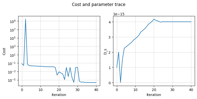
The DataFit class has an internal “cost-logger” attribute that can be used to log and visualize the cost function during optimization. This is useful for monitoring the progress of the optimization. The cost logger is a dictionary that stores the cost function value at each iteration. The cost logger can be accessed using the cost_logger attribute of the DataFit object.

By default, the cost logger just tracks the cost function value. DataFit.plot_trace can be used the plot the progress at the end of the optimization.

objective = iwp.objectives.CurrentDriven(data, options={"model": model})
current_driven = iwp.DataFit(objective, parameters=parameters)
params_fit = current_driven.run(params_for_pipeline)
current_driven.plot_trace()

[IDAS ERROR]  IDACalcIC
  The linesearch algorithm failed: step too small or too many backtracks.


[IDAS ERROR]  IDASolve
  At t = 0 and h = 8.88112e-60, the corrector convergence failed repeatedly or with |h| = hmin.

(<Figure size 800x400 with 2 Axes>,
 array([<Axes: xlabel='Iteration', ylabel='Cost'>,
        <Axes: xlabel='Iteration', ylabel='D_s'>], dtype=object))

The cost logger can be changed by passing the cost_logger argument to the DataFit object. For example, the following example shows how to pass a cost logger that plots the cost function and parameter values every 10 iterations.

current_driven = iwp.DataFit(
    objective,
    parameters=parameters,
    cost_logger=iwp.data_fits.CostLogger(plot_every=10),
)