Fitting diffusivity

In this example, we showcase some common workflows for fitting diffusion coefficients using pulse data.

import pybamm
import numpy as np
import pandas as pd
import ionworkspipeline as iwp
from scipy.integrate import cumulative_trapezoid
import matplotlib.pyplot as plt

0. Generate synthetic data

For this example, we set up a Single Particle Model with a stoichiometry dependent diffusivity. We first set up the model and parameters.

options = {"working electrode": "positive"}
model = pybamm.lithium_ion.SPM(options)
parameter_values = iwp.ParameterValues("Xu2019")


def D_p(sto, T):
    "NMC diffusivity from O'Regan et al. 2021"
    a1 = -0.9231
    a2 = -0.4066
    a3 = -0.993
    b1 = 0.3216
    b2 = 0.4532
    b3 = 0.8098
    c0 = -13.96
    c1 = 0.002534
    c2 = 0.003926
    c3 = 0.09924

    D = (
        10
        ** (
            c0
            + a1 * np.exp(-((sto - b1) ** 2) / c1)
            + a2 * np.exp(-((sto - b2) ** 2) / c2)
            + a3 * np.exp(-((sto - b3) ** 2) / c3)
        )
        * 2.7
    )

    return D


parameter_values.update({"Positive particle diffusivity [m2.s-1]": D_p})

# add the diffusivity as a variable for easy plotting later
sto = model.variables["Positive electrode stoichiometry"]
T = model.variables["Volume-averaged cell temperature [K]"]
model.variables["Positive particle diffusivity [m2.s-1]"] = D_p(sto, T)

We can plot what the diffusivity looks like as a function of stoichiometry

sto = pybamm.linspace(0, 1, 100)
_, ax = plt.subplots()
ax = pybamm.plot(sto, D_p(sto, 298.15), ax=ax)
ax.set_xlabel("Stoichiometry [-]")
ax.set_ylabel("Positive particle diffusivity [m2.s-1]")

Text(0, 0.5, 'Positive particle diffusivity [m2.s-1]')

Then we generate some synthetic data

parameters_for_data = parameter_values.copy()
experiment = pybamm.Experiment(
    [("Rest for 10s", "Discharge at C/10 for 5 minutes", "Rest for 30 minutes")] * 10,
    period="10 seconds",
)
sim = iwp.Simulation(model, parameter_values=parameters_for_data, experiment=experiment)
sim.solve(initial_soc=0.8)
variables = ["Time [s]", "Time [h]", "Current [A]", "Voltage [V]"]
data = pd.DataFrame(sim.solution.get_data_dict(variables))
data = data.rename(columns={"Cycle": "Cycle number", "Step": "Step number"})
t_h = data["Time [h]"].values
current = data["Current [A]"].values
data["Capacity [A.h]"] = cumulative_trapezoid(current, t_h, initial=0)

and plot the data.

sim.plot(
    [
        "Current [A]",
        "Voltage [V]",
        "Positive electrode stoichiometry",
        "Positive particle diffusivity [m2.s-1]",
    ]
)

<pybamm.plotting.quick_plot.QuickPlot at 0x74feeac560c0>

Because we are generating synthetic data, we can also obtain the electrode stoichiometry. However, in practice we would need to calculate this from the capacity and voltage data, as well as the parameterization of the open-circuit voltage. The following block shows how to calculate the stoichiometry from the data.

Note: this assumes we have already fitted the open-circuit potential and cell capacity, for example using the MSMRHalfCell model.

# Calculate initial stoichiometry from initial voltage based on the model OCP
V_init = data["Voltage [V]"].iloc[0]
sto_calc = iwp.calculations.InitialStoichiometryFromVoltageHalfCell("positive")
params_for_pipeline = parameter_values.copy()
params_for_pipeline.update(
    {"Initial voltage in positive electrode [V]": V_init}, check_already_exists=False
)
sto_params = sto_calc.run(params_for_pipeline)
sto_init = sto_params["Initial stoichiometry in positive electrode"]
# Calculate electrode capacity
param = pybamm.LithiumIonParameters(options={"working electrode": "positive"})
Q = params_for_pipeline.evaluate(param.p.prim.Q_init)
# Add stoichiometry to the data
data["Stoichiomety"] = sto_init + data["Capacity [A.h]"] / Q

1. Fitting a scalar across all pulses

The simplest assumption we can make is that the diffusivity takes a single scalar value across all pulses. We can fit this scalar value to the data.

In the following we set up an objective for each cycle, passing in the initial concentration using the custom_parameters argument of the objective function. Any values provided in the custom_parameter dictionary are passed the simulation in that objective only. We create a dictionary of objectives, using the mid-point stoichiometry as the keys.

# We fit a scalar for the diffusivity
parameters = {
    "Positive particle diffusivity [m2.s-1]": iwp.Parameter(
        "D_p", initial_value=1e-14, bounds=(1e-15, 1e-13)
    ),
}

# The model and solver are passed to the objective as options
options = {
    "model": model,
}

# We build a dictionary of objectives, indexed by the mid-point stoichiometry
# We pass in the initial concentration in the positive electrode as a custom parameter
# see the
c_max = parameter_values["Maximum concentration in positive electrode [mol.m-3]"]
objectives = {}
cycles = data["Cycle number"].unique()
for cycle in cycles:
    data_cycle = data[data["Cycle number"] == cycle]
    # Use tht initial stoichiometry as to set the initial concentration
    sto_init = data_cycle["Stoichiomety"].iloc[0]
    # Use midpoint stoichiometry as the stoichiometry for the cycle
    sto_final = data_cycle["Stoichiomety"].iloc[-1]
    mid_point_sto = (sto_init + sto_final) / 2
    # Create a new objective for each cycle
    objective = iwp.objectives.Pulse(
        data_cycle,
        options=options,
        custom_parameters={
            "Initial concentration in positive electrode [mol.m-3]": c_max * sto_init
        },
    )
    objectives[mid_point_sto] = objective

# And create the data fit object
scalar_data_fit = iwp.DataFit(objectives, parameters=parameters)

# make sure we're not accidentally initializing with the correct values by passing
# them in
params_for_pipeline = {k: v for k, v in parameter_values.items() if k not in parameters}

# Finally we run the fit
scalar_results = scalar_data_fit.run(params_for_pipeline)

Let’s plot the results.

_ = scalar_data_fit.plot_fit_results()

We can see the fit is reasonable, but not perfect. We know the diffusivity is stoichiometry dependent, so let’s look at some alternatives.

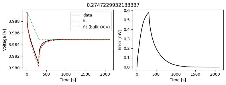
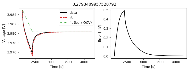
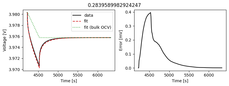
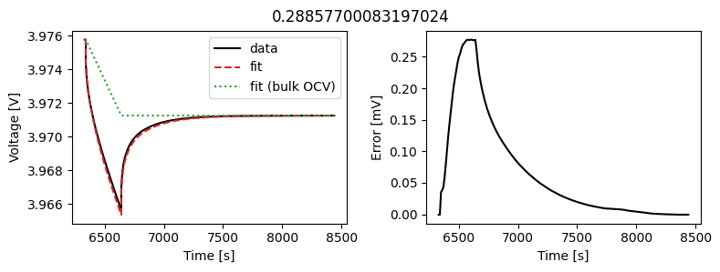
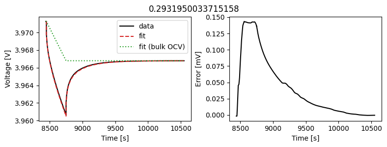
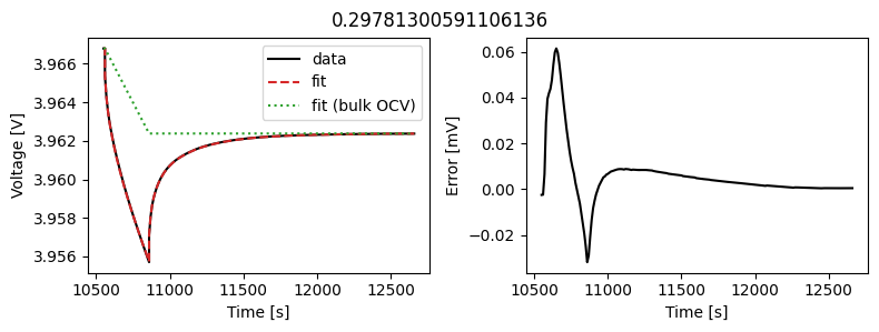
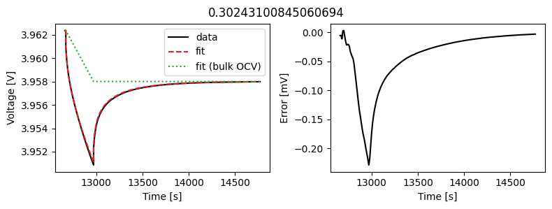
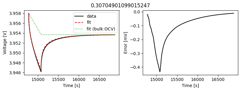
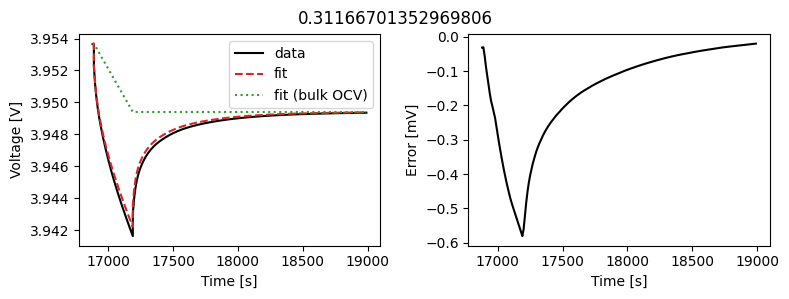
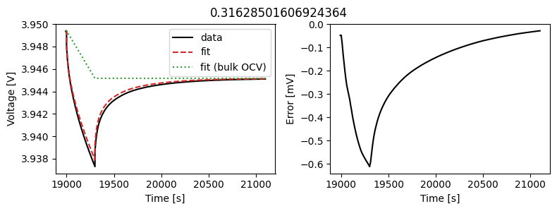
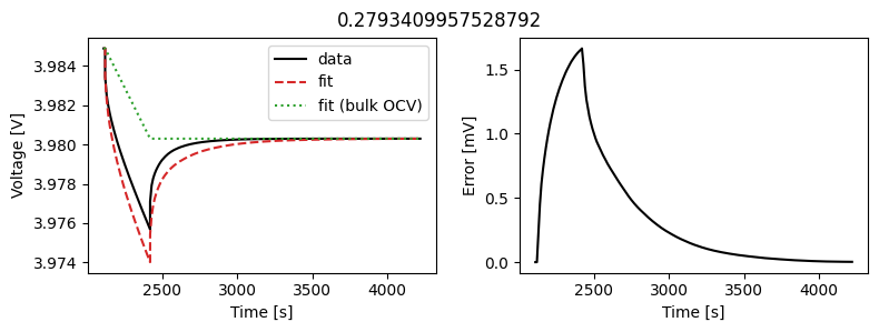
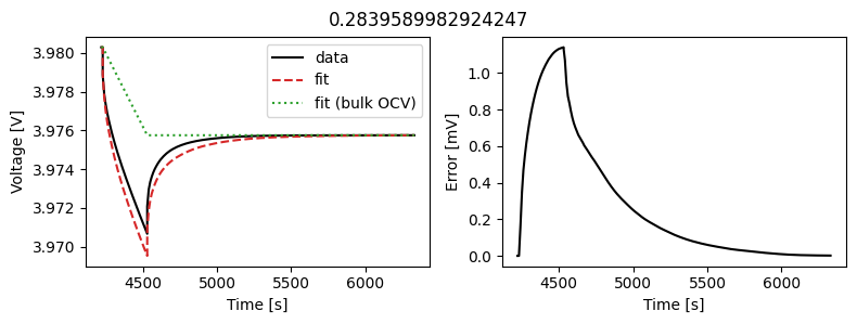
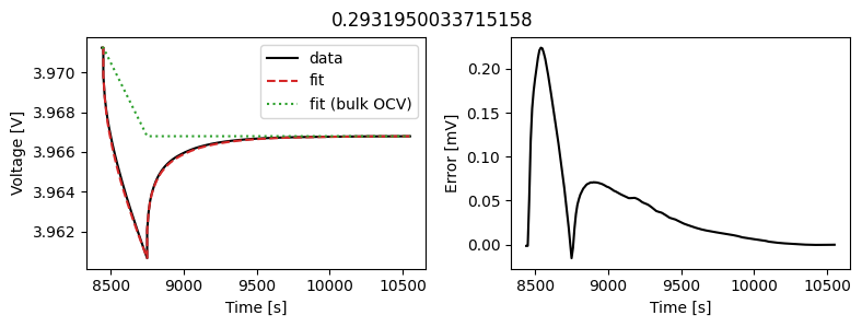
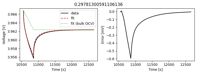
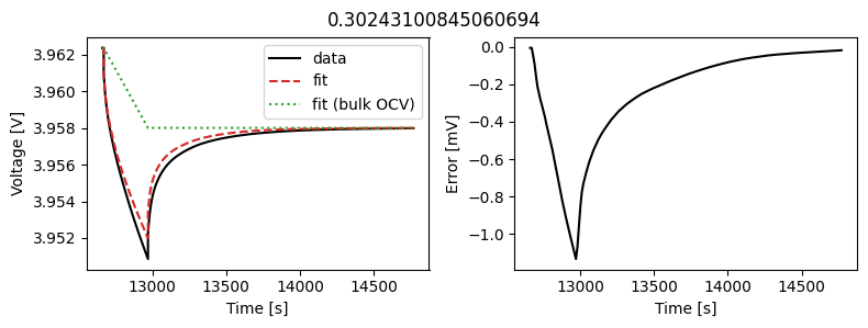
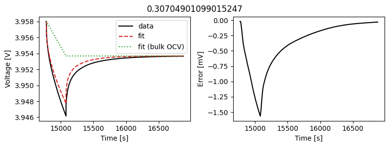
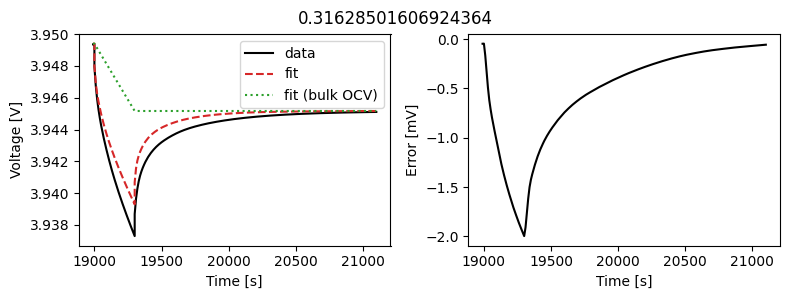
2. Fitting a scalar for each pulse

We can instead assume that the diffusivity is a scalar but fit a value for each pulse in the data. This could then be used to create an interpolant or used as the basis for fitting a function to the calculated diffusivity.

We can use the same objectives as before, but instead of setting up a DataFit object we use an ArrayDataFit object. This will fit the parameters separately for each objective in the dictionary.

array_data_fit = iwp.ArrayDataFit(objectives, parameters=parameters)
array_results = array_data_fit.run(params_for_pipeline)

Let’s plot the results

_ = array_data_fit.plot_fit_results()

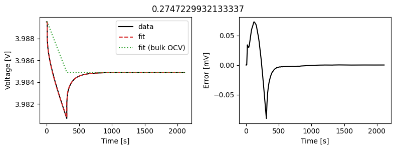
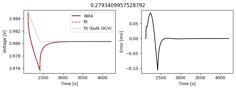
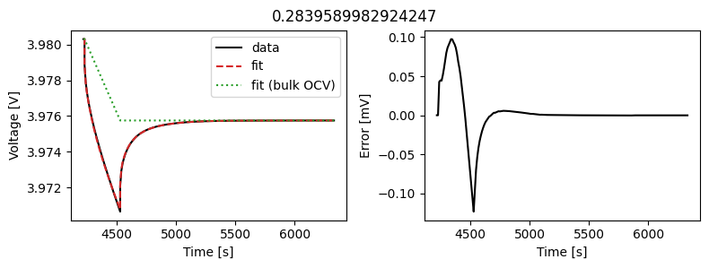
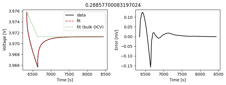
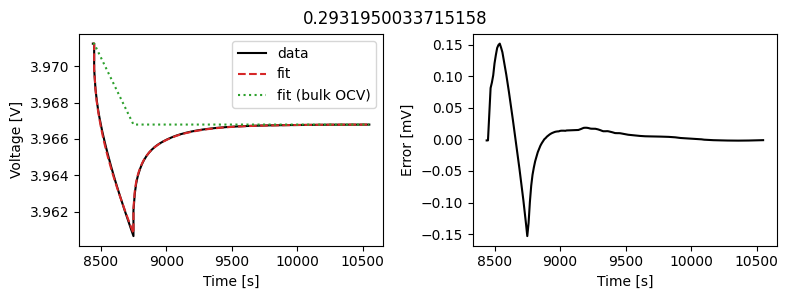
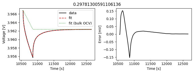
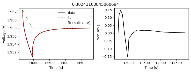
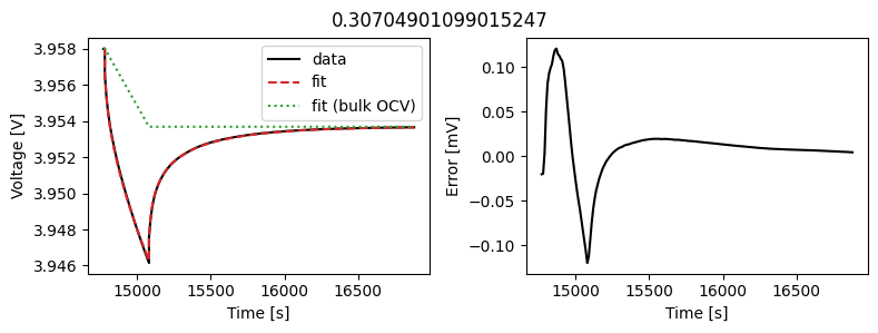
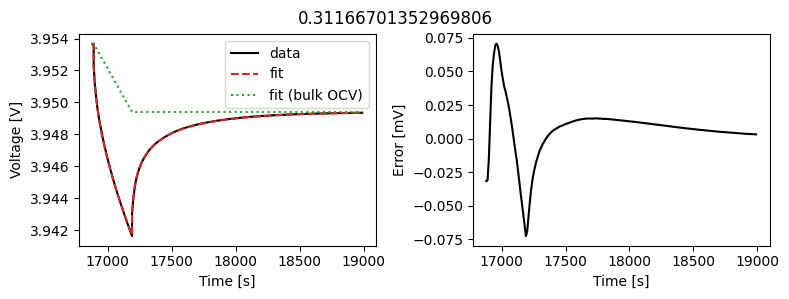
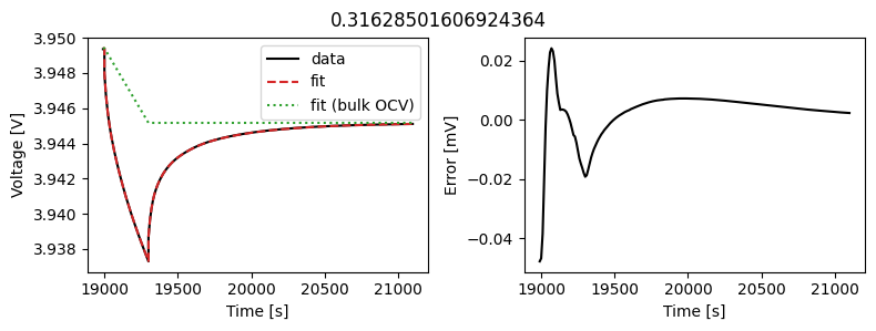
This results in a much better fit for each individual pulse.

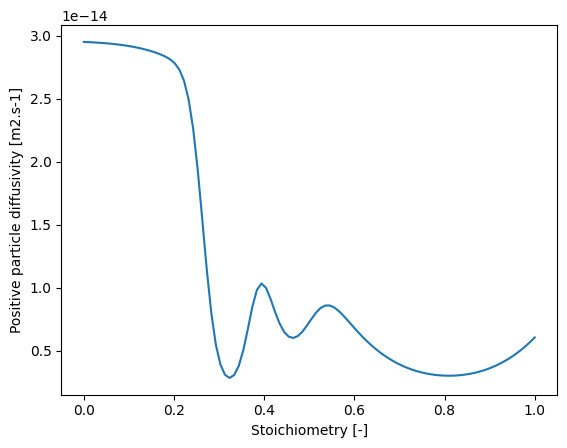
3. Calculating the diffusivity from each pulse

We can calculate the diffusivity from each pulse using an analytical formula. The below pipeline calculation using equation 26 of Wang, A. A., et al. “Review of parameterisation and a novel database (LiionDB) for continuum Li-ion battery models.” Progress in Energy 4.3 (2022).

# Create a dict to store sto vs diffusivity
sto_D_data = {"Stoichiometry": [], "Diffusivity [m2.s-1]": []}

# Loop over the cycles and calculate the diffusivity
for cycle in data["Cycle number"].unique():
    data_cycle = data[data["Cycle number"] == cycle]
    # Use midpoint stoichiometry as the stoichiometry for the cycle
    sto = (data_cycle["Stoichiomety"].iloc[-1] + data_cycle["Stoichiomety"].iloc[0]) / 2
    # Calculate the diffusivity
    calc_params_fit = iwp.calculations.DiffusivityFromPulse("positive", data_cycle).run(
        parameter_values
    )
    D = calc_params_fit["Positive particle diffusivity [m2.s-1]"]
    # Store the results
    sto_D_data["Stoichiometry"].append(sto)
    sto_D_data["Diffusivity [m2.s-1]"].append(D)

sto_D_data = pd.DataFrame(sto_D_data)

We can then create an interpolant from our computed stoichiometry vs. diffusivity data.

interpolant = iwp.calculations.DiffusivityDataInterpolant("positive", sto_D_data)
interp_params = interpolant.run({})
D_interp = interp_params["Positive particle diffusivity [m2.s-1]"]

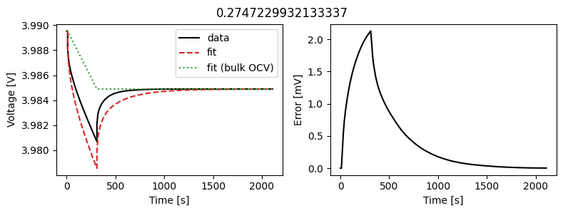
This approach often gives the correct “shape” for the stoichiometry dependent diffusivity, but the magnitude is often off. We can use this as a starting point for fitting a function to the data. In the following, we utilize the “scale factor” option which allows us to fit a scale factor that multiplies the calculated diffusivity.

# Define a new diffusivity function that scales the interpolated diffusivity
scaled_interpolant = iwp.calculations.DiffusivityDataInterpolant(
    "positive", sto_D_data, options={"scale factor": True}
)


# Set up the parameters for the fit
parameters = {
    "Positive particle diffusivity scale factor": iwp.Parameter(
        "D_scale", bounds=(0.1, 10)
    ),
}


# Create a pipeline that uses the interpolant and then fits the scale factor
scaled_interp_data_fit = iwp.DataFit(objectives, parameters=parameters)
pipeline = iwp.Pipeline(
    {
        "known values": iwp.direct_entries.DirectEntry(
            params_for_pipeline, "known values"
        ),
        "interpolant": scaled_interpolant,
        "fit": scaled_interp_data_fit,
    }
)
scaled_interp_params_fit = pipeline.run()

Finally, we plot the results.

_ = scaled_interp_data_fit.plot_fit_results()