Weighted cost functions

In this notebook, we show different ways to weight the cost function when combining multiple objectives and output variables.

import pybamm
import numpy as np
import pandas as pd
import ionworkspipeline as iwp
import matplotlib.pyplot as plt

Generate data

First, we generate some synthetic data using a variant of the Robertson model. We add an activation energy term to the rate constants of the reaction so that we can run the simulation at different temperatures (assuming isothermal conditions). To keep things simple, we ignore units and assume the system is written in a suitable non-dimensional form.

class Robertson(pybamm.BaseModel):
    def __init__(self):
        super().__init__()
        x = pybamm.Variable("x")
        y = pybamm.Variable("y")
        z = pybamm.Variable("z")

        k_1 = pybamm.Parameter("k_1")
        E_1 = pybamm.Parameter("E_1")
        k_2 = pybamm.Parameter("k_2")
        E_2 = pybamm.Parameter("E_2")
        k_3 = pybamm.Parameter("k_3")
        E_3 = pybamm.Parameter("E_3")
        T = pybamm.Parameter("T")

        arr_1 = pybamm.exp(-E_1 / T)
        arr_2 = pybamm.exp(-E_2 / T)
        arr_3 = pybamm.exp(-E_3 / T)

        self.rhs = {
            x: -k_1 * arr_1 * x + k_2 * arr_2 * y * z,
            y: k_1 * arr_1 * x - k_2 * arr_2 * y * z - k_3 * arr_3 * y**2,
            z: k_3 * arr_3 * y**2,
        }
        self.initial_conditions = {x: 1, y: 0, z: 0}
        self.variables = {"x": x, "y": y, "z": z}


model = Robertson()
true_inputs = {
    "k_1": 5,
    "E_1": 0.5,
    "k_2": 3,
    "E_2": 0.25,
    "k_3": 1.5,
    "E_3": 0.2,
    "T": pybamm.InputParameter("T"),
}
true_params = iwp.ParameterValues(true_inputs)
true_params.process_model(model)
solver = pybamm.IDAKLUSolver()
t_data = np.linspace(0, 10, 1000)
data_dict = {}
for T in [1, 10]:
    solution = solver.solve(model, t_eval=t_data, inputs={"T": T}, t_interp=t_data)
    x_data = solution["x"].data
    y_data = solution["y"].data
    z_data = solution["z"].data
    data = pd.DataFrame({"t": t_data, "x": x_data, "y": y_data, "z": z_data})
    data_dict[T] = data

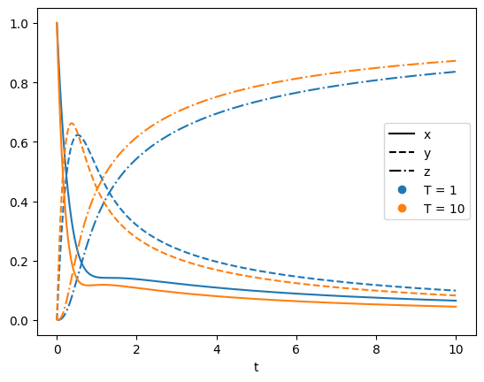
# Plot the data
colors = ["tab:blue", "tab:orange", "tab:green"]
for i, (T, data) in enumerate(data_dict.items()):
    plt.plot(data["t"], data["x"], "-", color=colors[i])
    plt.plot(data["t"], data["y"], "--", color=colors[i])
    plt.plot(data["t"], data["z"], "-.", color=colors[i])
    if i == 0:
        plt.plot([], [], "-", color="k", label="x")
        plt.plot([], [], "--", color="k", label="y")
        plt.plot([], [], "-.", color="k", label="z")
    plt.plot([], [], "o", color=colors[i], label=f"T = {T}")
plt.xlabel("t")
_ = plt.legend()

Fit model

To fit this model, we set up a custom Objective class which defines how the error function is calculated from the solution. Here we will compare the values of x, y, z between model and data. The cost function used to make the comparison can be specified later.

class Objective(iwp.objectives.Objective):
    def process_data(self):
        data = self.data["data"]
        self._processed_data = {"x": data["x"], "y": data["y"], "z": data["z"]}

    def build(self, all_parameter_values):
        data = self.data["data"]
        t_data = data["t"].values

        model = Robertson()
        all_parameter_values.process_model(model)
        self.simulation = iwp.Simulation(model, t_eval=t_data, t_interp=t_data)

    def run(self, inputs, full_output=False):
        sim = self.simulation
        sol = sim.solve(inputs=inputs)
        return {"x": sol["x"].data, "y": sol["y"].data, "z": sol["z"].data}

We create a dictionary of objectives to fit the data at each temperature. When we do this, we pass in the known temperature as a custom_parameter to the objective. This is a parameter that is not fitted, but is passed to the model when the objective is evaluated.

objectives = {}
for T, data in data_dict.items():
    objectives[T] = Objective(data, custom_parameters={"T": T})

We choose to use RMSE as our cost function. We can pass weights for both the objectives and variables to the Cost class. objective_weights should be a dictionary with the same keys as the objectives and the values are the weights for each objective. variable_weights should be a dictionary with the same keys as the variables and the values are the weights for each variable. If no weights are passed, the default is 1 for all objectives and variables.

objective_weights = {1: 1, 10: 1}
variable_weights = {"x": 0.1, "y": 0.1, "z": 0.8}
cost = iwp.costs.RMSE(
    objective_weights=objective_weights, variable_weights=variable_weights
)

We can then specify which parameters need to be fitted, which parameters are known, define bounds, and pass this to the standard DataFit class to fit the unknown parameters. Let’s assume we know \(k_2\) and \(E_2\) and fit the remaining parameters.

fit_parameters = {
    "k_1": iwp.Parameter("k_1", initial_value=1, bounds=(0, 10)),
    "E_1": iwp.Parameter("E_1", initial_value=0.1, bounds=(0, 1)),
    "k_3": iwp.Parameter("k_3", initial_value=1, bounds=(0, 10)),
    "E_3": iwp.Parameter("E_3", initial_value=0.1, bounds=(0, 1)),
}
known_parameters = {"k_2": 3, "E_2": 0.5}

optimizer = iwp.optimizers.ScipyMinimize()
data_fit = iwp.DataFit(
    objectives, parameters=fit_parameters, cost=cost, optimizer=optimizer
)
new_parameter_values = data_fit.run(known_parameters)

Let’s compare the fitted and true values of the parameters.

for key, value in new_parameter_values.items():
    print(f"{key}: {value:.4f} (fit) {true_params[key]:.4f} (true)")

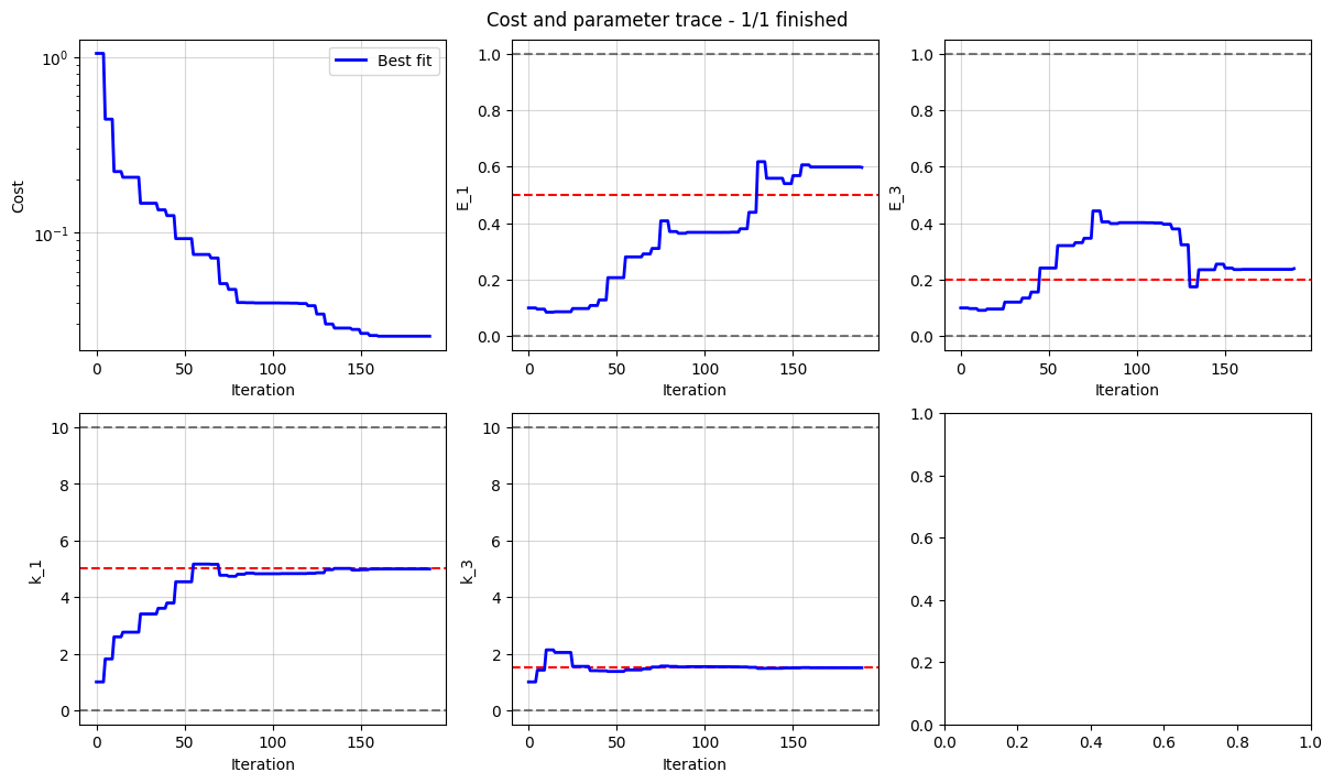
k_1: 4.9935 (fit) 5.0000 (true)
E_1: 0.5969 (fit) 0.5000 (true)
k_3: 1.5005 (fit) 1.5000 (true)
E_3: 0.2390 (fit) 0.2000 (true)

We can plot the trace of the cost and the parameter values to see how the fit progressed.

fig, axes = data_fit.plot_trace()
for ax, true_value in zip(
    axes[1:], [true_inputs[param.name] for param in data_fit.all_fit_parameters]
):
    ax.axhline(true_value, color="r", linestyle="--")