1. Half-cell OCP

In this example, we use synthetic GITT data to fit the MSMR model of the half-cell open-circuit potential (OCP) for a graphite electrode.

Before running this example, make sure to run the script true_parameters/generate_data.py to generate the synthetic data.

from pathlib import Path

import ionworkspipeline as iwp
import iwutil

MSMR model theory

Here we briefly outline the MSMR model, as described in Baker and Verbrugge (2018).

The MSMR model is developed by assuming that all electrochemical reactions at the electrode/electrolyte interface in a lithium insertion cell can be expressed in the form

\[ \text{Li}^{+} + \text{e}^{-} + \text{H}_{j} \rightleftharpoons (\text{Li--H})_{j}.\]

For each species \(j\), a vacant host site \(\text{H}_{j}\) can accommodate one lithium leading to a filled host site \((\text{Li--H})_{j}\). The OCV for this reaction is written as

\[ U_j = U_j^0 + \frac{\omega_j}{f}\log\left(\frac{X_j - x_j}{x_j}\right),\]

where \(f = F/(RT)\), and \(R\), \(T\), and \(F\) are the universal gas constant, temperature in Kelvin, and Faraday’s constant, respectively. Here \(X_j\) represents the total fraction of available host sites which can be occupied by species \(j\), \(x_j\) is the fraction of filled sites occupied by species \(j\), \(U_j^0\) is a concentration independent standard electrode potential, and the \(\omega_j\) is an unitless parameter that describes the level of disorder of the reaction represented by gallery \(j\). Alternatively, the model can be expressed in terms of the fractional capacities \(Q_j\) instead of the fractional site occupancies \(X_j\), with \(Q_j = X_j Q_{tot}\), \(q_j = x_j Q_{tot}\) and \(Q_{tot}\) the total capacity of the electrode.

The equation for each reaction can be inverted to give

\[x_j = \frac{X_j}{1+\exp[f(U-U_j^0)/\omega_j]}.\]

The overall electrode state of charge is given by summing the fractional occupancies

\[x = \sum_j x_j = \sum_j \frac{X_j}{1+\exp[f(U-U_j^0)/\omega_j]},\]

which is an explicit closed form expression for the inverse of the OCV. This is opposite to many battery models where one typically gives the OCV as an explicit function of the state of charge (or stoichiometry).

At a particle interface with the electrolyte, local equilibrium requires that

\[U_j = U(x) \quad \forall j.\]

Load the data

We load the synthetic GITT data for the negative electrode and the extract the OCP from the relaxed voltages.

gitt_data = iwutil.read_df(
    Path("synthetic_data") / "half_cell_negative_electrode" / "gitt.csv"
)
ocp_data = iwp.data_fits.preprocess.pulse_data_to_ocp(gitt_data)

Set up the parameters to fit

We first set up our initial guesses for the parameters. For the MSMR model, good initial guesses can be found manually by looking at the data (e.g. dVdQ analysis) or by using the built-in function iwp.objectives.msmr_half_cell_initial_guess.

Let’s firs set up some initial guesses manually to get a feel for how the parameter values affect the model. We need to specify initial values for \(U_j\), \(X_j\), and \(\omega_j\), as well as the total capacity of the electrode. We can also specify a “lower excess capacity” parameter, which is the amount of capacity that is not accessed in the experiment at the lower end of the stoichiometry. In practice, the electrode will no be fully delithiated at the start of the experiment - this parameter describes the amount of capacity required to fully delithiate the electrode from its initial state in the experiment.

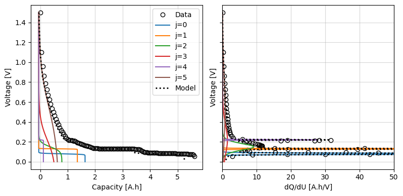
We can use the iwp.objectives.plot_each_species_msmr function to help with this. This function plots the OCP and dQ/dU for each reaction. Each reaction has a corresponding peak in the dQ/dU curve, so we can use this to help us pick reasonable initial values.

Try changing the initial values and re-running the cell to see how the model changes.

Q_use = ocp_data["Capacity [A.h]"].max()
param_init = {
    "U0_n_0": 0.08,
    "X_n_0": 0.30,
    "w_n_0": 0.1,
    "U0_n_1": 0.13,
    "X_n_1": 0.25,
    "w_n_1": 0.04,
    "U0_n_2": 0.15,
    "X_n_2": 0.15,
    "w_n_2": 0.9,
    "U0_n_3": 0.22,
    "X_n_3": 0.11,
    "w_n_3": 4.1,
    "U0_n_4": 0.22,
    "X_n_4": 0.03,
    "w_n_4": 0.05,
    "U0_n_5": 0.55,
    "X_n_5": 0.13,
    "w_n_5": 8.5,
    "Negative electrode capacity [A.h]": Q_use,
    "Negative electrode lower excess capacity [A.h]": 0.01 * Q_use,
}
fig, ax = iwp.objectives.plot_each_species_msmr(
    ocp_data, param_init, "negative", voltage_limits=(0, 1.5)
)
ax[1].set_xlim(0, 50)

/home/docs/checkouts/readthedocs.org/user_builds/ionworks-ionworkspipeline/envs/v0.6.6/lib/python3.12/site-packages/ionworkspipeline/data_fits/objectives/ocp_msmr_util.py:153: RuntimeWarning: overflow encountered in exp
  qj = Qj / (1 + np.exp(f * (U_lin - U0) / w))

(0.0, 50.0)

Alteratively, we can can use the iwp.objectives.msmr_half_cell_initial_guess to automatically generate initial guesses. This function works by using a Gaussian Mixture Model to cluster the dQ/dU curve and then using the peak of each cluster as an initial guess for the reaction parameters. The user must specify the number of reactions to fit.

num_reactions = 6
gmm_param_init = iwp.objectives.msmr_half_cell_initial_guess(
    "negative", ocp_data, num_reactions
)

Next we use these initial guesses to set up the parameters for the fit. Each of the fit parameters must be an iwp.Parameter object, which has a name, initial value, and bounds. We can create these objects manually, for example:

a = iwp.Parameter("a", initial_value=1.0, bounds=(0, 2))

but for the MSMR model, we can use the iwp.objectives.get_msmr_params_for_fit function to automatically create these objects. The function takes the electrode name and initial guesses, and returns a dictionary of iwp.Parameter objects. Additional keyword arguments, such as a bounds_function that specifies how to set the bounds for the parameters, can be passed to the function to give more control over the fitting process.

Here we use the “Qj” format, where the capacity of each reaction is a fit parameter, rather than the fractional site occupancies \(X_j\). Note this function does not add the lower excess capacity parameter, so we need to do this separately.

parameters = iwp.objectives.get_msmr_params_for_fit(
    param_init, "negative", Q_use, species_format="Qj"
)
# Add the lower excess capacity parameter
parameters.update(
    {
        "Negative electrode lower excess capacity [A.h]": (
            iwp.Parameter(
                "Q_lowex", initial_value=0.01 * Q_use, bounds=(0, 0.2 * Q_use)
            )
        )
    }
)

Run the workflow

Now we are ready to run the workflow. To run the workflow with the default settings, we can use the fit_plot_save function. This function runs the fit, saves the results (if a save_dir keyword argument is provided), and plots the results. All of the workflows have a common interface, where you typically need to provide the data, the parameters to be fitted, and a dictionary of known parameters. In the case of half-cell workflows, we also need to specify the electrode name (“negative” or “positive”).

Here, the only known parameter is the ambient temperature, which we set to 25°C. This should be the temperature at which the experiment was conducted.

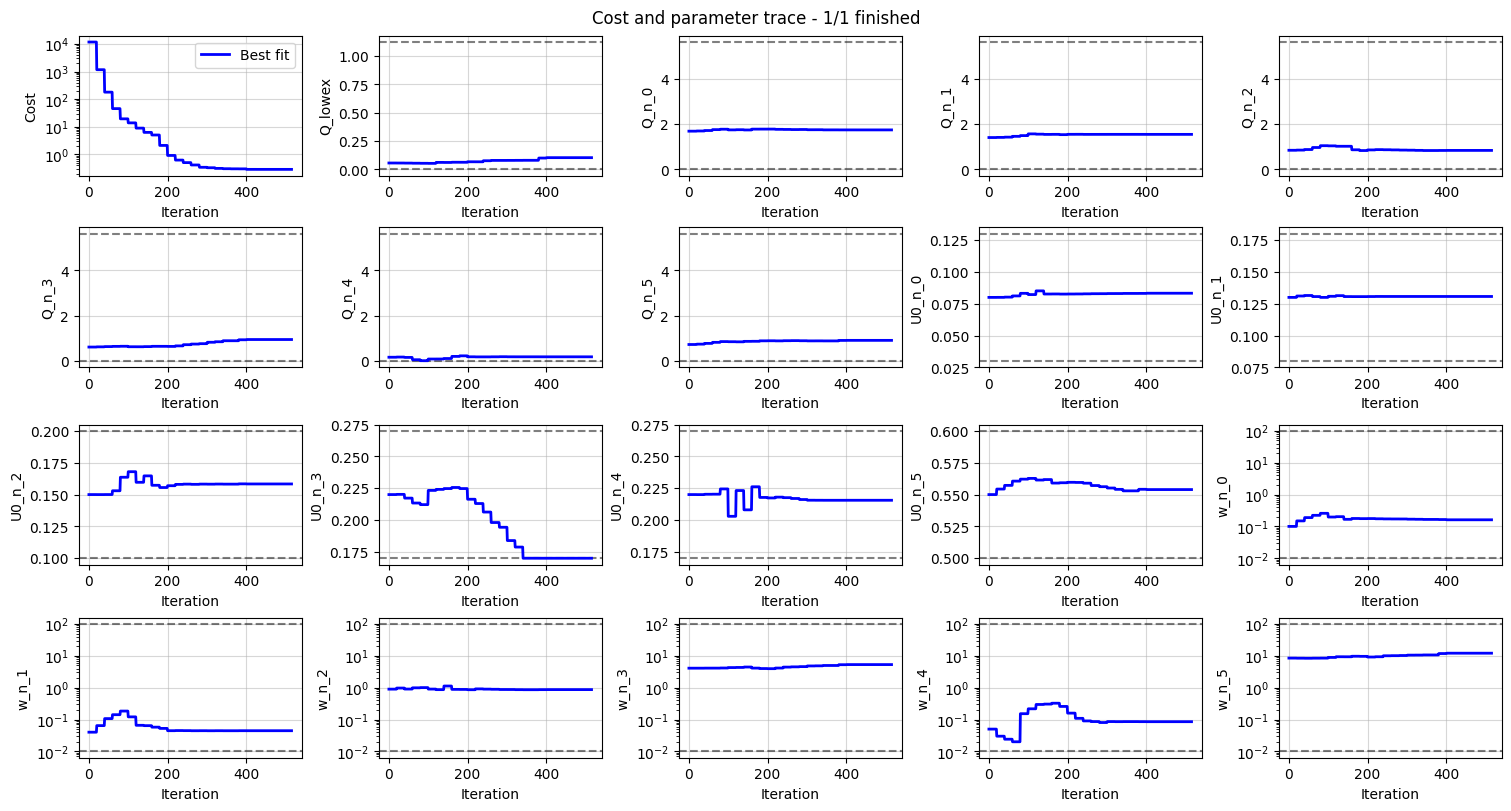
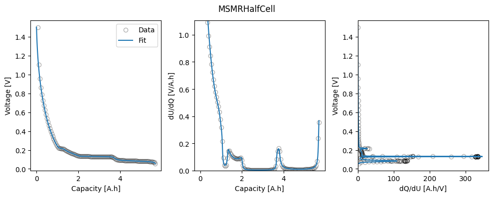
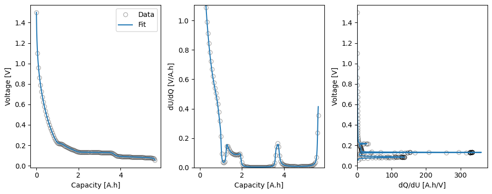
The workflow returns a Results object, which contains the fitted parameters, and a dictionary of figures with the keys “trace” and the name of the objective function (in this case “MSMRHalfCell”). The trace figure shows the evolution of the cost function and parameter values during the fit. The MSMRHalfCell figure shows the fitted OCP, dU/dQ and dQ/dU curves.

known_params = {"Ambient temperature [K]": 298.15}
objective_kwargs = {
    "options": {"model": iwp.data_fits.models.MSMRHalfCellModel("negative")}
}
res, figs = iwp.workflows.half_cell_ocp.fit_plot_save(
    "negative",
    ocp_data,
    parameters,
    known_params,
    objective_kwargs=objective_kwargs,
)

/home/docs/checkouts/readthedocs.org/user_builds/ionworks-ionworkspipeline/envs/v0.6.6/lib/python3.12/site-packages/pybamm/expression_tree/binary_operators.py:260: RuntimeWarning: overflow encountered in square
  return left**right

We can take a look at the fitted parameters by accessing the parameter_values attribute of the Results object.

res.parameter_values

{'U0_n_0': 0.08464921259976635,
 'Q_n_0': 1.718508021569275,
 'w_n_0': 0.12489783514485973,
 'U0_n_1': 0.13067205412028754,
 'Q_n_1': 1.5362512878040553,
 'w_n_1': 0.04245802858652098,
 'U0_n_2': 0.15624301251386916,
 'Q_n_2': 0.8969683752619332,
 'w_n_2': 0.9420841197182819,
 'U0_n_3': 0.170000009290669,
 'Q_n_3': 1.0505739416898607,
 'w_n_3': 5.470209677642589,
 'U0_n_4': 0.21546742466504173,
 'Q_n_4': 0.18266632463024302,
 'w_n_4': 0.07419420605425898,
 'U0_n_5': 0.5999996625260607,
 'Q_n_5': 0.6455967634956143,
 'w_n_5': 8.798858986943193,
 'X_n_0': 0.28496635107011314,
 'X_n_1': 0.25474418409319977,
 'X_n_2': 0.14873704499224374,
 'X_n_3': 0.17420821953413104,
 'X_n_4': 0.03029008613281631,
 'X_n_5': 0.10705411417749608,
 'Negative electrode capacity [A.h]': 6.030564714450981,
 'Negative electrode lower excess capacity [A.h]': 0.015468819002568397}

What’s going on? A lower-level interface

The workflows are designed to be simple to use and cover most use cases. They can be customized by passing additional keyword arguments. For example, we can pass a dictionary datafit_kwargs to specify the cost function or optimizer to be used in the fit. Much more customization is possible by accessing the underlying DataFit and Optimizer classes directly. Here we will go through the steps of running the fit manually.

We can use the same parameters and known_params as dicitonaries as before, but we need to create the Objective and DataFit objects manually.

Let’s start by creating the objective function. We use the MSMRHalfCell objective function and pass in the electrode and the data. Here, we can also specify any additional options that we want to use in the fit or pass in callbacks to interact with the fitting process, for example to configure custom plots or logging. Here we will pass a “dUdQ cutoff” option, that tells the objective to ignore the data above a certain dU/dQ value. We use the calculate_dUdQ_cutoff function to calculate this value from the data, based on some reasonable default settings.

dUdQ_cutoff = iwp.data_fits.util.calculate_dUdQ_cutoff(ocp_data)
objective = iwp.objectives.MSMRHalfCell(
    ocp_data,
    options={
        "dUdQ cutoff": dUdQ_cutoff,
        "model": iwp.data_fits.models.MSMRHalfCellModel("negative"),
    },
)

After we’ve created the objective, we can create the DataFit object. The DataFit object takes in the objective and the parameters to fit. We can also customize the fitting processing by passing in a cost function and selecting an optimizer.

cost = iwp.costs.Difference()
optimizer = iwp.optimizers.ScipyLeastSquares(verbose=1)
datafit = iwp.DataFit(objective, parameters=parameters, cost=cost, optimizer=optimizer)

Finally, we run the fit and plot the results.

results = datafit.run(known_params)
_ = datafit.plot_trace()
_ = datafit.plot_fit_results()

`xtol` termination condition is satisfied.
Function evaluations 41, initial cost 5.8659e+03, final cost 1.4440e-01, first-order optimality 5.73e-01.