Data Fit example
This notebook shows how the DataFit class works via examples. For design principles, see the user_guide. For detailed documentation on the DataFit class, see the API reference.
Simple non-battery example
The Ionworks battery parameter pipeline is built around PyBaMM models. We’ll begin the demonstration of the DataFit class by creating a simple dynamical model that we will use to generate and fit synthetic data.
import pybamm
import numpy as np
import pandas as pd
import ionworkspipeline as iwp


class LotkaVolterra(pybamm.BaseModel):
    def __init__(self):
        super().__init__()
        x = pybamm.Variable("x")
        y = pybamm.Variable("y")

        a = pybamm.Parameter("a")
        b = pybamm.Parameter("b")
        c = pybamm.Parameter("c")
        d = pybamm.Parameter("d")

        self.rhs = {x: a * x - b * x * y, y: -c * y + d * x * y}
        self.initial_conditions = {x: 2, y: 1}
        self.variables = {"x": x, "y": y}


model = LotkaVolterra()
true_inputs = {"a": 1.5, "b": 0.5, "c": 3.0, "d": 0.3}
true_params = iwp.ParameterValues(true_inputs)
true_params.process_model(model)
solver = pybamm.ScipySolver()
t_data = np.linspace(0, 10, 1000)
solution = solver.solve(model, t_data)

# extract data and add noise
x_data = solution["x"].data + 0.1 * np.random.rand(t_data.size)
y_data = solution["y"].data + 0.1 * np.random.rand(t_data.size)

data = pd.DataFrame({"t": t_data, "x": x_data, "y": y_data})
To fit this model, we set up a custom Objective class that defines how the error function is calculated from the solution.
class Objective(iwp.objectives.Objective):
    def process_data(self):
        data = self.data["data"]
        self._processed_data = {"x": data["x"], "y": data["y"]}

    def build(self, all_parameter_values):
        data = self.data["data"]
        t_data = data["t"].values

        model = LotkaVolterra()
        all_parameter_values.process_model(model)
        self.simulation = iwp.Simulation(model, t_eval=t_data, t_interp=t_data)

    def run(self, inputs, full_output=False):
        sim = self.simulation
        sol = sim.solve(inputs=inputs)
        return {"x": sol["x"].data, "y": sol["y"].data}


objective = Objective(data)
We can then specify the parameters that need to be fitted, identify any known parameters (none in this case), define bounds, and pass these specifications to the standard DataFit class to fit the unknown parameters.
fit_parameters = {
    "a": iwp.Parameter("a", bounds=(0, np.inf)),
    "b": iwp.Parameter("b", bounds=(0, np.inf)),
    "c": iwp.Parameter("c", bounds=(0, np.inf)),
    "d": iwp.Parameter("d", bounds=(0, np.inf)),
}
known_parameters = {}

optimizer = iwp.optimizers.ScipyLeastSquares(verbose=2)
data_fit = iwp.DataFit(objective, parameters=fit_parameters, optimizer=optimizer)
new_parameter_values = data_fit.run(known_parameters)
   Iteration     Total nfev        Cost      Cost reduction    Step norm     Optimality
       0              1         2.1190e+03                                    5.57e+02
       1              3         1.8882e+03      2.31e+02       3.56e-01       4.44e+02
       2              4         1.6345e+03      2.54e+02       7.06e-01       2.85e+03
       3              5         1.2492e+03      3.85e+02       3.96e-01       1.70e+03
4 6 2.2835e+02 1.02e+03 7.09e-01 6.64e+03
       5              8         9.7346e+01      1.31e+02       2.28e-01       1.68e+03
       6              9         6.9293e+01      2.81e+01       4.63e-01       6.88e+03
       7             10         1.5185e+00      6.78e+01       2.59e-01       8.93e+02
       8             11         2.1555e-01      1.30e+00       1.74e-02       2.32e+01
       9             12         2.1495e-01      6.03e-04       5.73e-04       1.12e-01
      10             13         2.1495e-01      1.29e-08       1.59e-06       6.02e-04
      11             14         2.1495e-01      2.86e-13       7.74e-09       8.23e-06
Both `ftol` and `xtol` termination conditions are satisfied.
Function evaluations 14, initial cost 2.1190e+03, final cost 2.1495e-01, first-order optimality 8.23e-06.
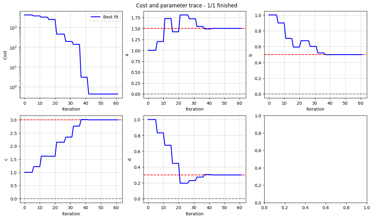
We then plot the trace of the cost and the parameter values to see how the fit progressed.
fig, axes = data_fit.plot_trace()
for ax, true_value in zip(axes[1:], true_inputs.values()):
    ax.axhline(true_value, color="r", linestyle="--")
We can reuse the same Objective and DataFit class but change which parameters are known and which are to be fitted. This flexibility is useful for battery models where we want to fit only a subset of the parameters to experimental data while keeping other parameters fixed.
fit_parameters = {
    "a": iwp.Parameter("a", bounds=(0, np.inf)),
    "b": iwp.Parameter("b", bounds=(0, np.inf)),
}
known_parameters = {"c": 3, "d": 0.3}

data_fit = iwp.DataFit(objective, parameters=fit_parameters, optimizer=optimizer)
new_parameter_values = data_fit.run(known_parameters)

for k, v in new_parameter_values.items():
    true = true_inputs[k]
    print(f"Parameter {k}: true: {true:.3f}, fitted: {v:.3f}")
   Iteration     Total nfev        Cost      Cost reduction    Step norm     Optimality
       0              1         2.6436e+03                                    9.69e+02
       1              2         2.5958e+03      4.78e+01       5.15e-01       1.04e+03
       2              3         2.5800e+03      1.58e+01       3.27e-02       1.26e+03
       3              4         2.5562e+03      2.38e+01       1.75e-02       1.51e+03
       4              5         2.5198e+03      3.65e+01       2.23e-02       1.82e+03
       5              6         2.4629e+03      5.69e+01       3.00e-02       2.21e+03
       6              7         2.3706e+03      9.23e+01       4.23e-02       2.74e+03
       7              8         2.2104e+03      1.60e+02       6.29e-02       3.52e+03
       8              9         1.9008e+03      3.10e+02       1.00e-01       4.76e+03
       9             10         1.2536e+03      6.47e+02       1.77e-01       6.05e+03
      10             11         3.5411e+02      8.99e+02       3.33e-01       9.41e+02
      11             12         3.1267e+01      3.23e+02       3.64e-01       3.31e+03
      12             13         2.7983e-01      3.10e+01       1.83e-02       7.25e+01
      13             14         2.1629e-01      6.35e-02       2.63e-03       2.94e-01
      14             15         2.1629e-01      2.71e-07       3.03e-06       1.12e-03
      15             16         2.1629e-01      3.41e-12       9.03e-09       8.60e-06
Both `ftol` and `xtol` termination conditions are satisfied.
Function evaluations 16, initial cost 2.6436e+03, final cost 2.1629e-01, first-order optimality 8.60e-06.
Parameter a: true: 1.500, fitted: 1.500
Parameter b: true: 0.500, fitted: 0.498
Battery example: constant-current experiment
We now repeat the same procedure for a battery model. We start by creating a model and solving it to generate synthetic data.
model = pybamm.lithium_ion.SPM()
parameter_values = iwp.ParameterValues("Chen2020")
sim = iwp.Simulation(model, parameter_values=parameter_values)
t = np.linspace(0, 3600, 1000)
sim.solve([0, 3600], t_interp=t)
data = pd.DataFrame(
    {x: sim.solution[x].entries for x in ["Time [s]", "Current [A]", "Voltage [V]"]}
)
Next, we set up which parameters are to be fitted, and call the pre-defined CurrentDriven objective function, which solves the model with the current from the data and calculates the error between voltage from the model and the data.
# In this example we just fit the diffusivity in the positive electrode
parameters = {
    "Positive particle diffusivity [m2.s-1]": iwp.Parameter("D_s", initial_value=1e-15),
}

objective = iwp.objectives.CurrentDriven(data, options={"model": model})
current_driven = iwp.DataFit(objective, parameters=parameters)

# make sure we're not accidentally initializing with the correct values by passing
# them in
params_for_pipeline = {k: v for k, v in parameter_values.items() if k not in parameters}

results = current_driven.run(params_for_pipeline)

print(
    f"True parameter value: {parameter_values['Positive particle diffusivity [m2.s-1]']:.3e}"
)
print(
    f"Fitted parameter value: {results['Positive particle diffusivity [m2.s-1]']:.3e}"
)
[IDAS ERROR]  IDASolve
  At t = 0 and h = 8.88113e-60, the corrector convergence failed repeatedly or with |h| = hmin.
True parameter value: 4.000e-15
Fitted parameter value: 4.000e-15
The results variable is a Result class which contains information about the optimization. The optimal parameter values are accessible by indexing the solution, like
results['Positive particle diffusivity [m2.s-1]']
or through its properties,
parameter_values: The final values of the optimized parameters.optimizer_result: The result object returned by the optimizer.callbacks: The callbacks used during optimization.children: Results from multistarted parameter estimation (if multistart was used).
results.parameter_values
{'Positive particle diffusivity [m2.s-1]': 3.999999784435016e-15}
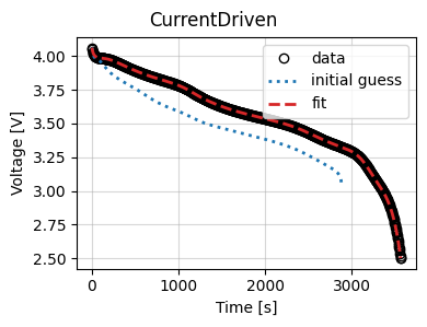
We can also plot the fit results.
current_driven.plot_fit_results()
{'CurrentDriven': [(<Figure size 400x300 with 1 Axes>,
   <Axes: xlabel='Time [s]', ylabel='Voltage [V]'>)]}