Fitting features in GITT data

In this example, we show how to extract features from GITT data to be used in objective functions instead of directly fitting the data. We use the features defined in “Bayesian parameterization of continuum battery models from featurized electrochemical measurements considering noise.”, Kuhn et al., 2023.

import pybamm
import pandas as pd
import ionworkspipeline as iwp
import matplotlib.pyplot as plt
from matplotlib.patches import FancyArrowPatch
from scipy.integrate import cumulative_trapezoid
from functools import partial

Generate data

We begin by generating synthetic data for a half-cell. For this example, we simply generate a few cycles of a GITT experiment.

model = pybamm.lithium_ion.SPM({"working electrode": "positive"})

parameter_values = iwp.ParameterValues("Xu2019")


def j0(c_e, c_s_surf, c_s_max, T):
    j0_ref = pybamm.Parameter(
        "Positive electrode reference exchange-current density [A.m-2]"
    )
    c_e_init = pybamm.Parameter("Initial concentration in electrolyte [mol.m-3]")

    return (
        j0_ref
        * (c_e / c_e_init) ** 0.5
        * (c_s_surf / c_s_max) ** 0.5
        * (1 - c_s_surf / c_s_max) ** 0.5
    )


parameter_values.update(
    {
        "Positive electrode reference exchange-current density [A.m-2]": 5,
        "Positive electrode exchange-current density [A.m-2]": j0,
        "Positive particle diffusivity [m2.s-1]": 1e-14,
    },
    check_already_exists=False,
)

C_rate = 1 / 15
pause_h = 30 / 60 / 60
step_h = 0.1
rest_h = 0.2
V_min = parameter_values["Lower voltage cut-off [V]"]
V_max = parameter_values["Upper voltage cut-off [V]"]
experiment = pybamm.Experiment(
    [
        (
            f"Rest for {pause_h} hour (1 second period)",
            f"Discharge at {C_rate} C for {step_h} hour or until {V_min} V (1 second period)",
            f"Rest for {rest_h} hour (1 second period)",
        ),
    ]
    * 3
)

sim = iwp.Simulation(model, parameter_values=parameter_values, experiment=experiment)
_ = sim.solve()

We save the results to a dataframe.

variables = ["Time [s]", "Time [h]", "Current [A]", "Voltage [V]"]
df = pd.DataFrame(sim.solution.get_data_dict(variables))
df = df.rename(columns={"Cycle": "Cycle number", "Step": "Step number"})
t_h = df["Time [h]"].values
currents = df["Current [A]"].values
Q = cumulative_trapezoid(currents, t_h, initial=0)
df["Capacity [A.h]"] = Q

Extracting features

Next we extract the features from the data and save them to a dataframe using the function iwp.objectives.pulse.gitt_features_objective_variables. When doing so, we pass in the step numbers which correspond to the pulse and rest steps.

Let’s look at the features of the first cycle.

data = df[df["Cycle number"] == 0]
data["Overpotential [mV]"] = (data["Voltage [V]"] - data["Voltage [V]"].iloc[0]) * 1000

pulse_step_num = 1
gitt_features = iwp.objectives.pulse.gitt_features_objective_variables(
    data,
    step_nums=[pulse_step_num],
    full_output=True,
)

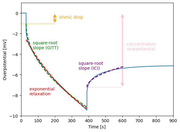
We then plot the features against the synthetic data.

fig, ax = plt.subplots()

# plot overpotential during the pulse and rest steps
t = data["Time [s]"].values
eta = data["Overpotential [mV]"].values
ax.plot(t, eta)

# plot the GITT features

# ohmic drop
eta_r = gitt_features["U0_gitt_step_1"][0]
x_loc = 200
ax.add_artist(
    FancyArrowPatch(
        (x_loc, eta_r),
        (x_loc, 0),
        arrowstyle="<->",
        color="orange",
        mutation_scale=15,
        linewidth=2,
    )
)
ax.hlines(eta_r, xmin=t[0], xmax=x_loc, color="orange", linestyle=":")
ax.annotate("ohmic drop", (x_loc + 25, eta_r / 2), color="orange")

# square-root slope (GITT)
t_gitt = gitt_features["t_gitt_step_1"]
U_gitt = gitt_features["U_gitt_step_1"]
ax.plot(t_gitt, U_gitt, color="green", linestyle="--", linewidth=2)
ax.annotate("square-root \nslope (GITT)", (70, -3.5), color="green")

# exponential relaxation
t_exp = gitt_features["t_exp_step_1"]
U_exp = gitt_features["U_exp_step_1"]
ax.plot(t_exp, U_exp, color="red", linestyle="--", linewidth=2)
ax.annotate("exponential \nrelaxation", (50, -8), color="red")

# square-root slope (ICI)
t_ici = gitt_features["t_ici_step_1"]
U_ici = gitt_features["U_ici_step_1"]
ax.plot(t_ici, U_ici, color="purple", linestyle="--", linewidth=2)
ax.annotate("square-root \nslope (ICI)", (340, -5.5), color="purple")

# concentration overpotential
eta_c = gitt_features["U0_ici_step_1"][0]
x_loc = 600
ax.add_artist(
    FancyArrowPatch(
        (x_loc, eta_c),
        (x_loc, 0),
        arrowstyle="<->",
        color="pink",
        mutation_scale=15,
        linewidth=2,
    )
)
ax.hlines(eta_c, xmin=t_ici[0], xmax=x_loc, color="pink", linestyle=":")
ax.annotate("concentration \noverpotential", (x_loc + 25, eta_c / 2), color="pink")

ax.set_xlim([0, 900])
ax.set_ylim([-10, 1])
ax.set_xlabel("Time [s]")
ax.set_ylabel("Overpotential [mV]")

Text(0, 0.5, 'Overpotential [mV]')

Fitting the features

To use these features when fitting data, we can pass the function gitt_features_objective_variable to the Pulse objective class using the objective variables key in the options dictionary. Any keyword arguments can be passed to the function using the objective_variables_kwargs key in the options dictionary. Other useful objective variables functions include overpotential_objective_variables, which calculates the overpotentials at the specified times, and ici_features_objective_variables, which calculates the features for the Intermittent Current Interruption experiment (see “Implementing intermittent current interruption into Li-ion cell modelling for improved battery diagnostics.”, Yin et al., 2022 for details).

Let’s compare fitting the features with fitting the data directly.

parameters = {
    "Positive particle diffusivity [m2.s-1]": iwp.Parameter(
        "D_s", initial_value=1e-14, bounds=(5e-15, 5e-13)
    ),
    "Positive electrode reference exchange-current density [A.m-2]": iwp.Parameter(
        "j0", initial_value=5, bounds=(0.1, 10)
    ),
}
parameters_for_pipeline = {
    k: v for k, v in parameter_values.items() if k not in parameters.keys()
}

objective_variables_fns = [
    iwp.objectives.pulse.voltage_objective_variables,
    partial(
        iwp.objectives.pulse.gitt_features_objective_variables, step_nums=[1]
    ),  # pulse step
]
params_fit_list = []
for objective_variables_fn in objective_variables_fns:
    objectives = iwp.objectives.pulse.get_pulse_objectives_by_cycle(
        data,
        options={
            "model": model,
            "objective variables": objective_variables_fn,
        },
    )
    gitt_half_cell = iwp.DataFit(objectives, parameters=parameters)
    results = gitt_half_cell.run(parameters_for_pipeline)
    params_fit_list.append(results)
    print(results)

    gitt_half_cell.plot_fit_results()

Result(
  Positive particle diffusivity [m2.s-1]: 1e-14
  Positive electrode reference exchange-current density [A.m-2]: 5
)

Result(
  Positive particle diffusivity [m2.s-1]: 1.26935e-14
  Positive electrode reference exchange-current density [A.m-2]: 0.1
)

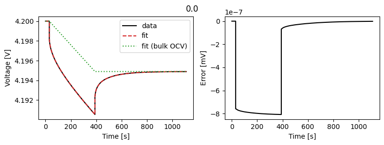
For synthetic data, fitting the voltage directly gives better results than fitting the features. However, in practice, fitting the features can be more robust to noise and other model or experimental errors.