Fitting LAM in composite electrodes

In this example, we show how to use the MSMR model to fit the capacity of different materials in a composite electrode. We generate synthetic half-cell data for a composite electrode with two materials in a fresh and aged state and use the MSMR model to fit the capacity of each material in the aged data.

import pybamm
import ionworkspipeline as iwp
import matplotlib.pyplot as plt
import numpy as np
import pandas as pd

We generate synthetic data by specifying the capacity of the graphite and silicon in the composite. Let’s define the base parameter values and a function to generate the synthetic data.

# Specify MSMR parameters with the total graphite and silicon capacities left as parameters
# that can be varied
gr_cap = pybamm.Parameter("Graphite capacity [A.h]")
si_cap = pybamm.Parameter("Silicon capacity [A.h]")
parameter_values = {
    # MSMR parameters - graphite
    "U0_n_0": 0.08843467036305873,
    "Q_n_0": 0.43336 * gr_cap,
    "w_n_0": 0.08624582794789712,
    "U0_n_1": 0.12798999719375143,
    "Q_n_1": 0.23963 * gr_cap,
    "w_n_1": 0.08027331262623288,
    "U0_n_2": 0.14330798736501915,
    "Q_n_2": 0.15018 * gr_cap,
    "w_n_2": 0.7251288122409935,
    "U0_n_3": 0.170820726326599,
    "Q_n_3": 0.05462 * gr_cap,
    "w_n_3": 2.5206592503098726,
    "U0_n_4": 0.21446035430385701,
    "Q_n_4": 0.06744 * gr_cap,
    "w_n_4": 0.0948564197626504,
    "U0_n_5": 0.3607980467134248,
    "Q_n_5": 0.05476 * gr_cap,
    "w_n_5": 6.133684065785475,
    # MSMR parameters - silicon
    "U0_n_6": 0.12522011472333466,
    "Q_n_6": 0.21834 * si_cap,
    "w_n_6": 0.10933476524461729,
    "U0_n_7": 0.1842071161944969,
    "Q_n_7": 0.23264 * si_cap,
    "w_n_7": 0.16781090721088374,
    "U0_n_8": 0.14648529724013823,
    "Q_n_8": 0.42492 * si_cap,
    "w_n_8": 0.5746396954282488,
    "U0_n_9": 0.4698932042915728,
    "Q_n_9": 0.12410 * si_cap,
    "w_n_9": 1.0155683156057957,
    "Ambient temperature [K]": 298.15,
    "Negative electrode lower excess capacity [A.h]": 0,
    "Negative electrode capacity [A.h]": gr_cap + si_cap,
}


def generate_data(parameter_values, gr_cap, si_cap):
    # Add capacity values to parameter_values
    parameter_values = parameter_values.copy()
    parameter_values["Graphite capacity [A.h]"] = gr_cap
    parameter_values["Silicon capacity [A.h]"] = si_cap

    # Get capacity as a function of voltage
    n_species = len([k for k in parameter_values.keys() if "U0_n" in k])
    q_n_fun = iwp.objectives.get_q_half_cell_msmr(
        n_species, "negative", species_format="Qj"
    )
    U_n = np.linspace(1.5, 0.01, 1000)
    q_n = (
        iwp.ParameterValues(parameter_values)
        .process_symbol(q_n_fun(U_n))
        .evaluate()
        .flatten()
    )
    data = pd.DataFrame({"Capacity [A.h]": q_n, "Voltage [V]": U_n})

    return data

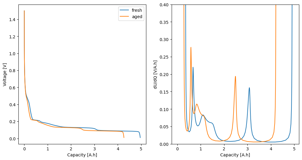
In this example, the fresh cell has a total capacity of 5 Ah, and silicon makes up 20% of the capacity of the composite. We generate aged data for a composite where the graphite capacity has reduced to 3.8 Ah and the silicon capacity has reduced to 0.5 Ah.

fresh_gr_cap, fresh_si_cap = 4, 1
fresh_data = generate_data(parameter_values, fresh_gr_cap, fresh_si_cap)
aged_gr_cap, aged_si_cap = 3.8, 0.5
aged_data = generate_data(parameter_values, aged_gr_cap, aged_si_cap)

Next we plot the “data”.

fig, ax = plt.subplots(1, 2, figsize=(12, 6))
for label, data in zip(["fresh", "aged"], [fresh_data, aged_data]):
    q = data["Capacity [A.h]"]
    U = data["Voltage [V]"]
    dUdQ = -np.gradient(U, q)
    ax[0].plot(q, U, label=label)
    ax[1].plot(q, dUdQ, label=label)
ax[0].set_xlabel("Capacity [A.h]")
ax[0].set_ylabel("Voltage [V]")
ax[0].legend()
ax[1].set_xlabel("Capacity [A.h]")
ax[1].set_ylabel("dU/dQ [V/A.h]")
ax[1].set_ylim(0, 0.4)

(0.0, 0.4)

Now we will use the MSMR model to fit the total capacity of each material in the composite in the aged data. We will assume that the reference potentials \(U^0_j\) and the order parameters \(\omega_j\) are the same as in the fresh data. We also assume that the site fractions \(X_j = Q_j / Q\), where \(Q\) is the total capacity, stay the same. In practice different degradation mechanisms may affect the MSMR parameters differently.

For the capacity parameters we use the fresh parameter values as an initial guess (in practice we would have fit these to fresh cell data first)

Q_use = aged_data["Capacity [A.h]"].max()
parameters = {
    "Graphite capacity [A.h]": iwp.Parameter(
        "Q_gr", initial_value=fresh_gr_cap, bounds=(0, Q_use)
    ),
    "Silicon capacity [A.h]": iwp.Parameter(
        "Q_si", initial_value=fresh_si_cap, bounds=(0, Q_use)
    ),
}

We set up and run the MSMR fit

# set up the half-cell MSMR objective and data fit
options = {
    "model": iwp.data_fits.models.MSMRHalfCellModel("negative"),
}
objective = iwp.objectives.MSMRHalfCell(
    aged_data,
    options=options,
)
ocp_msmr = iwp.DataFit(objective, parameters=parameters)

# The MSMRHalfCell objective expects both the Xj and Qj parameters, so we add them to the
# parameter_values dictionary before fitting.
parameter_values.update(iwp.objectives.msmr_Qj_to_Xj(parameter_values, "negative"))

# Run the fit, passing in the known parameter values (we only fit Q_gr and Q_si)
results = ocp_msmr.run(parameter_values)

/home/docs/checkouts/readthedocs.org/user_builds/ionworks-ionworkspipeline/envs/v0.6.6/lib/python3.12/site-packages/pybamm/expression_tree/binary_operators.py:260: RuntimeWarning: overflow encountered in square
  return left**right

and plot the results.

_ = ocp_msmr.plot_fit_results()

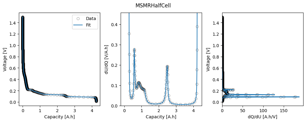
We can calculate the capacity of each material in the aged data by summing the capacity of each reaction that corresponds to that material.

gr_cap = results["Graphite capacity [A.h]"]
si_cap = results["Silicon capacity [A.h]"]
print(f"Fitted Graphite capacity: {gr_cap} A.h")
print(f"Fitted Silicon capacity: {si_cap} A.h")

Fitted Graphite capacity: 3.797200461942198 A.h
Fitted Silicon capacity: 0.5020158923990075 A.h

We see that the fit values agree well with the values used to generate the aged data.

In this example, we have used the MSMR model to fit the capacity of different materials in a composite electrode. However, a similar approach could be used on full cell data using the MSMRFullCell objective instead.