Multistart

Multistart is an optimization approach that initiates multiple runs from different starting points within the search space. This technique is particularly useful for navigating complex, non-convex problems, as it reduces the likelihood of getting stuck in local optima.

Pros of Multistart:

• Avoids local minima: Increases the likelihood of locating a global solution.

• Improves fitting reliability: Testing from multiple initial points can yield more robust results.

• Parallelization-friendly: Independent starting points allow for efficient computation on multiple cores.

• Useful for non-convex problems: Aids in exploring complex, high-dimensional spaces which are common with battery models.

In this example, we will use the multistart to fit a model to synthetic data. We begin by creating a two-parameter oscillatory model.

import pybamm
import numpy as np
import pandas as pd
import ionworkspipeline as iwp
import matplotlib.pyplot as plt


class WavyModel(pybamm.BaseModel):
    def __init__(self):
        super().__init__()
        x = pybamm.Variable("x")

        t = pybamm.t

        omega_1 = pybamm.Parameter("Frequency 1 [Hz]")
        omega_2 = pybamm.Parameter("Frequency 2 [Hz]")

        self.rhs = {x: -x * (pybamm.Sin(omega_1 * t) + pybamm.Cos(omega_2 * t))}
        self.initial_conditions = {x: 1}
        self.variables = {"x": x}


model = WavyModel()
true_inputs = {
    "Frequency 1 [Hz]": 3,
    "Frequency 2 [Hz]": 0.1,
}

true_params = iwp.ParameterValues(true_inputs)
true_params.process_model(model)
solver = pybamm.IDAKLUSolver()
t_data = np.linspace(0, 10, 1000)

solution = solver.solve(model, [0, 10], t_interp=t_data)
x_data = solution["x"].data
data = pd.DataFrame({"t": t_data, "x": x_data})

Next, we create the Objective class.

class Objective(iwp.objectives.Objective):
    def process_data(self):
        data = self.data["data"]
        self._processed_data = {"t": data["t"].values, "x": data["x"].values}

    def build(self, all_parameter_values):
        data = self.data["data"]
        t_data = data["t"].values

        model = WavyModel()
        all_parameter_values.process_model(model)
        self.simulation = iwp.Simulation(model)

        self.simulation.set_t_eval([t_data[0], t_data[-1]])
        self.simulation.set_t_interp(t_data)

    def run(self, inputs, full_output=False):
        sim = self.simulation
        sol = sim.solve(inputs=inputs)
        return {"x": sol["x"].data}


objective = Objective(data)

Next, we define the parameters to fit and their bounds. Multistart calculates new initial guess for each simulation, so bounds must be provided for all parameters.

fit_parameters = {
    "Frequency 1 [Hz]": iwp.Parameter(
        "Frequency 1 [Hz]", initial_value=1, bounds=(0, 5)
    ),
    "Frequency 2 [Hz]": iwp.Parameter(
        "Frequency 2 [Hz]", initial_value=1, bounds=(0, 5)
    ),
}
known_parameters = {}

Then, we set up the DataFit object, which takes the objective function, the parameters to fit, and the optimizer as inputs. Here we set 15 multistarts and set a seed of 0 for reproducibility. By default, multistart uses numerous CPU cores to run simulations in parallel. This may be disabled by setting num_workers = 1.

data_fit = iwp.DataFit(
    objective,
    multistarts=15,
    options={"seed": 0},
    parameters=fit_parameters,
    optimizer=iwp.optimizers.ScipyMinimize(),
)

Now, we run the DataFit class and compare the best results with their true value.

results = data_fit.run(known_parameters)
for k, v in results.items():
    print(f"{k}: {true_inputs[k]:.5e} (true) {v:.5e} (fit)")

Frequency 1 [Hz]: 3.00000e+00 (true) 3.00000e+00 (fit)
Frequency 2 [Hz]: 1.00000e-01 (true) 1.00000e-01 (fit)

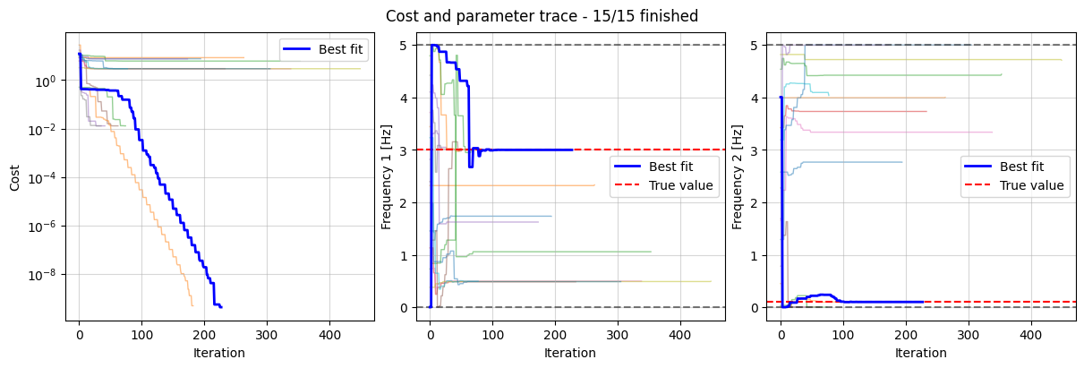
We can plot the trace of each individual optimization run. Each line represents a single optimization run. The best result is represented by the solid blue line whose cost has the smallest value after completing the simulation.

Many optimizations become stuck in local minima. With enough multistarts, we can still find the true solution.

fig, axes = data_fit.plot_trace()
for ax, true_value in zip(
    axes[1:], [true_inputs[param.name] for param in data_fit.all_fit_parameters]
):
    ax.axhline(true_value, color="r", linestyle="--", label="True value")
    ax.legend(loc="right")

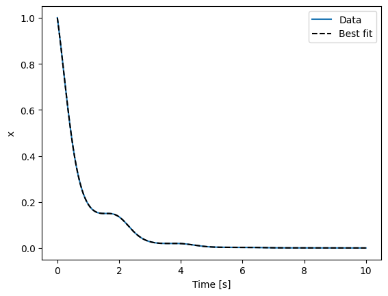
Finally, we plot the results.

fig, ax = plt.subplots()

fit = objective.run(results.parameter_values)
ax.plot(data["t"], data["x"], label="Data")
ax.plot(data["t"], fit["x"], "--", label="Best fit", color="black")

ax.set_xlabel("Time [s]")
ax.set_ylabel("x")
ax.legend()

<matplotlib.legend.Legend at 0x7a362f72a270>

The results for each multistart run are accessible using the children property of the results.

results.children

[Result(
   Frequency 1 [Hz]: 1.73425
   Frequency 2 [Hz]: 2.76545
 ),
 Result(
   Frequency 1 [Hz]: 2.33124
   Frequency 2 [Hz]: 4.00143
 ),
 Result(
   Frequency 1 [Hz]: 3.00542
   Frequency 2 [Hz]: 0
 ),
 Result(
   Frequency 1 [Hz]: 0.486008
   Frequency 2 [Hz]: 3.73336
 ),
 Result(
   Frequency 1 [Hz]: 3.00542
   Frequency 2 [Hz]: 0
 ),
 Result(
   Frequency 1 [Hz]: 3.00542
   Frequency 2 [Hz]: 0
 ),
 Result(
   Frequency 1 [Hz]: 0.497481
   Frequency 2 [Hz]: 3.33727
 ),
 Result(
   Frequency 1 [Hz]: 3.00542
   Frequency 2 [Hz]: 5.64718e-09
 ),
 Result(
   Frequency 1 [Hz]: 0.494177
   Frequency 2 [Hz]: 4.71108
 ),
 Result(
   Frequency 1 [Hz]: 0.49619
   Frequency 2 [Hz]: 4.03954
 ),
 Result(
   Frequency 1 [Hz]: 0.487427
   Frequency 2 [Hz]: 4.99992
 ),
 Result(
   Frequency 1 [Hz]: 3
   Frequency 2 [Hz]: 0.1
 ),
 Result(
   Frequency 1 [Hz]: 1.05804
   Frequency 2 [Hz]: 4.44208
 ),
 Result(
   Frequency 1 [Hz]: 3
   Frequency 2 [Hz]: 0.1
 ),
 Result(
   Frequency 1 [Hz]: 1.62378
   Frequency 2 [Hz]: 5
 )]