3. Cycling data

In this example, we show how to use full-cell cycling data to fit model parameters. Specifically, we will fit the negative electrode reference exchange-current density. The workflow shown in this example is very general and can take any cycling data and fit the model to any collected data. Typically we fit the voltage and/or temperature.

Before running this example, make sure to run the script true_parameters/generate_data.py to generate the synthetic data.

from pathlib import Path

import ionworkspipeline as iwp
import iwutil
import pybamm

from true_parameters.parameters import full_cell

Load the data

This workflow can fit across multiple data at once. Here we will fit the time vs voltage data collected from three constant current experiments. We load the data into a dictionary whose keys are the C-rates.

data = {}
for rate in [0.1, 0.5, 1]:
    data[f"{rate} C"] = iwutil.read_df(
        Path("synthetic_data") / "full_cell" / f"{str(rate).replace('.', '_')}C.csv"
    )

Set up the parameters to fit

Now we set up our initial guesses and bounds for the parameters. As in the previous example, we create a dictionary of Parameter objects. We assume a symmetric Butler-Volmer exchange-current density. We create a function for the exchange-current density and fit a scalar reference exchange-current density.

def j0_n(c_e, c_s_surf, c_s_max, T):
    j0_ref = pybamm.Parameter(
        "Negative electrode reference exchange-current density [A.m-2]"
    )
    alpha = 0.5
    c_e_ref = 1000

    return (
        j0_ref
        * (c_e / c_e_ref) ** (1 - alpha)
        * (c_s_surf / c_s_max) ** alpha
        * (1 - c_s_surf / c_s_max) ** (1 - alpha)
    )


parameters = {
    "Negative electrode exchange-current density [A.m-2]": j0_n,
    "Negative electrode reference exchange-current density [A.m-2]": iwp.Parameter(
        "j0_n [A.m-2]",
        initial_value=8,
        bounds=(0.1, 10),
    ),
}

Get the known parameters

In this example, we assume we already know all of the model parameters except for the negative electrode diffusivity and reference exchange-current density. We load the known parameters from the true parameters script.

true_params = full_cell()
known_params = {k: v for k, v in true_params.items() if k not in parameters}

Run the workflow

Now we are ready to run the workflow. To run the workflow with the default settings, we can use the fit_plot_save function. This function runs the fit, saves the results (if a save_dir keyword argument is provided), and plots the results. All of the workflows have a common interface, where you typically need to provide the data, the parameters to be fitted, and a dictionary of known parameters.

Here we use the “current-driven” workflow, which takes the input current from the data and fits the model output to the objective variables specified by the user. By default it fits the voltage. In the case where data is a dictionary of multiple data sets, the simultaneously optimizes across all data.

As well as passing the data, parameters, and known parameters, we can pass additional keyword arguments to customize the fit. Here we pass a dictionary objective_kwargs to specify the model to use. Here we use the SPMe model. If no model is specified, an error is raised. We remove the events from the model to avoid triggering the voltage cut-off event.

For this workflow, we also use a the custom_parameters keyword argument, which allows us to pass additional parameters to the objective function that are specific to each objective. Here we use the custom_parameters to set the initial concentration in each electrode to match the initial voltage in the data, assuming the cell is at equilibrium at the start of each experiment. We can use the built-in initial_concentration_from_voltage function to calculate the initial concentration in each electrode. This function takes the cell type (“half” or “full”) and the electrode (“negative” or “positive”) as inputs, and calculates the initial concentration based on the voltage using the function pybamm.lithium_ion.get_initial_stoichiometries.

model = pybamm.lithium_ion.SPMe()
model.events = []
options = {"model": model}

custom_parameters = {
    "Initial concentration in negative electrode [mol.m-3]": iwp.data_fits.custom_parameters.initial_concentration_from_voltage(
        "full", "negative"
    ),
    "Initial concentration in positive electrode [mol.m-3]": iwp.data_fits.custom_parameters.initial_concentration_from_voltage(
        "full", "positive"
    ),
}
objective_kwargs = {"options": options}
res, figs = iwp.workflows.current_driven.fit_plot_save(
    data,
    parameters,
    known_params,
    objective_kwargs=objective_kwargs,
)

We can take a look at the fitted parameters by accessing the parameter_values attribute of the Results object.

res.parameter_values

{'Negative electrode exchange-current density [A.m-2]': <function __main__.j0_n(c_e, c_s_surf, c_s_max, T)>,
 'Negative electrode reference exchange-current density [A.m-2]': 0.6670080514922756}

What’s going on? A lower-level interface

The workflows are designed to be simple to use and cover most use cases. They can be customized by passing additional keyword arguments. For example, we can pass a dictionary datafit_kwargs to specify the cost function or optimizer to be used in the fit. Much more customization is possible by accessing the underlying DataFit and Optimizer classes directly. Here we will go through the steps of running the fit manually.

We can use the same parameters and known_params as dicitonaries as before, but we need to create the Objective and DataFit objects manually.

Let’s start by creating the objective function(s). We use the CurrentDriven objective function and pass in the data and model. Since we are fitting multiple data sets, we create a corresponding dictionary of Objective objects. We can use the same options and custom_parameters as before.

objectives = {}
for this_name, this_data in data.items():
    objectives[this_name] = iwp.objectives.CurrentDriven(
        this_data, options=options, custom_parameters=custom_parameters
    )

Next we create the DataFit object. Here we can also specify the cost function and optimizer to be used in the fit.

cost = iwp.costs.RMSE()
optimizer = iwp.optimizers.ScipyMinimize(method="Nelder-Mead")
datafit = iwp.DataFit(objectives, parameters=parameters, cost=cost, optimizer=optimizer)

Finally, we run the fit and plot the results.

results = datafit.run(known_params)
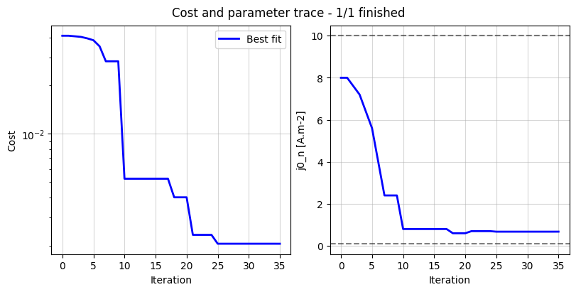
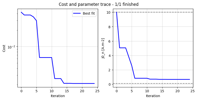
_ = datafit.plot_trace()
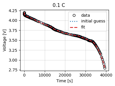
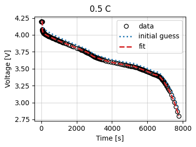
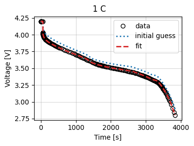
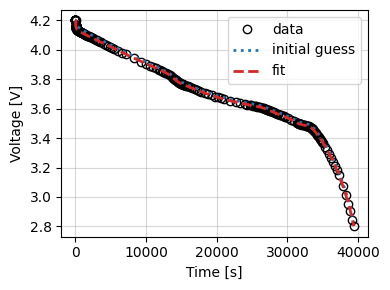
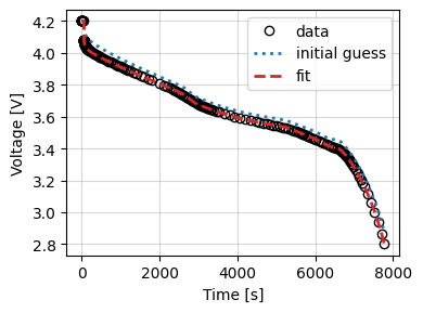
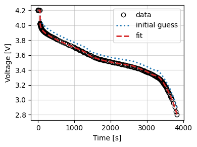
_ = datafit.plot_fit_results()