Using callbacks in objectives

This notebook explains how to use a callback in an objective function. For details on the Callback class, see the API reference. Potential use cases for this are:

• Plotting some outputs at each iteration of the optimization

• Saving internal variables to plot once the optimization is complete

Some objectives have “internal callbacks” which are not intended to be user facing. These are standard callbacks that can be used to plot the results of an optimization by using DataFit.plot_fit_results(). For user-facing callbacks, users should create their own callback objects and call them directly for plotting, as demonstrated in this notebook.

Creating a custom callback

To implement a custom callback, create a class that inherits from iwp.callbacks.Callback and calls some specific functions. See the documentation for iwp.callbacks.Callback for more information on the available functions and their expected inputs.

import ionworkspipeline as iwp
import matplotlib.pyplot as plt
import pybamm
import numpy as np
import pandas as pd

class MyCallback(iwp.callbacks.Callback):
    def __init__(self):
        super().__init__()
        # Implement our own iteration counter
        self.iter = 0

    def on_objective_build(self, logs):
        self.data_ = logs["data"]

    def on_run_iteration(self, logs):
        # Print some information at each iteration
        inputs = logs["inputs"]
        V_model = logs["outputs"]["Voltage [V]"]
        V_data = self.data_["Voltage [V]"]

        # calculate RMSE, note this is not necessarily the cost function used in the optimization
        rmse = np.sqrt(np.nanmean((V_model - V_data) ** 2))

        print(f"Iteration: {self.iter}, Inputs: {inputs}, RMSE: {rmse}")
        self.iter += 1

    def on_datafit_finish(self, logs):
        self.fit_results_ = logs

    def plot_fit_results(self):
        """
        Plot the fit results.
        """
        data = self.data_
        fit = self.fit_results_["outputs"]

        fit_results = {
            "data": (data["Time [s]"], data["Voltage [V]"]),
            "fit": (fit["Time [s]"], fit["Voltage [V]"]),
        }

        markers = {"data": "o", "fit": "--"}
        colors = {"data": "k", "fit": "tab:red"}
        fig, ax = plt.subplots()
        for name, (t, V) in fit_results.items():
            ax.plot(
                t,
                V,
                markers[name],
                label=name,
                color=colors[name],
                mfc="none",
                linewidth=2,
            )
        ax.grid(alpha=0.5)
        ax.set_xlabel("Time [s]")
        ax.set_ylabel("Voltage [V]")
        ax.legend()

        return fig, ax

To use this callback, we generate synthetic data for a current-driven experiment and fit a SPM using the CurrentDriven objective.

model = pybamm.lithium_ion.SPM()
parameter_values = iwp.ParameterValues("Chen2020")
t = np.linspace(0, 3600, 1000)
sim = iwp.Simulation(model, parameter_values=parameter_values, t_eval=t, t_interp=t)
sim.solve()
data = pd.DataFrame(
    {x: sim.solution[x].entries for x in ["Time [s]", "Current [A]", "Voltage [V]"]}
)

# In this example we just fit the diffusivity in the positive electrode
parameters = {
    "Positive particle diffusivity [m2.s-1]": iwp.Parameter("D_s", initial_value=1e-15),
}

# Create the callback
callback = MyCallback()
objective = iwp.objectives.CurrentDriven(
    data, options={"model": model}, callbacks=callback
)
current_driven = iwp.DataFit(objective, parameters=parameters)

# make sure we're not accidentally initializing with the correct values by passing
# them in
params_for_pipeline = {k: v for k, v in parameter_values.items() if k not in parameters}

_ = current_driven.run(params_for_pipeline)

Iteration: 0, Inputs: {'D_s': 1.0}, RMSE: 0.1590962387090109
Iteration: 1, Inputs: {'D_s': 1.0}, RMSE: 0.1590962387090109
Iteration: 2, Inputs: {'D_s': 2.0}, RMSE: 0.06447715147449944
Iteration: 3, Inputs: {'D_s': 0.0}, RMSE: 9999999996.444777
Iteration: 4, Inputs: {'D_s': 1.500000000015711}, RMSE: 0.10181491874308411
Iteration: 5, Inputs: {'D_s': 2.25}, RMSE: 0.05119216091393636
Iteration: 6, Inputs: {'D_s': 2.35}, RMSE: 0.04656550635368896
Iteration: 7, Inputs: {'D_s': 2.45}, RMSE: 0.042257479014892255
Iteration: 8, Inputs: {'D_s': 2.5500000000000003}, RMSE: 0.038236917252211275
Iteration: 9, Inputs: {'D_s': 2.6500000000000004}, RMSE: 0.03447343630136959
Iteration: 10, Inputs: {'D_s': 2.79142135623731}, RMSE: 0.029546608066060426
Iteration: 11, Inputs: {'D_s': 2.89142135623731}, RMSE: 0.026302653676153486
Iteration: 12, Inputs: {'D_s': 2.99142135623731}, RMSE: 0.02324787681904026
Iteration: 13, Inputs: {'D_s': 3.13284271247462}, RMSE: 0.019212560615620752
Iteration: 14, Inputs: {'D_s': 3.33284271247462}, RMSE: 0.014012802298131509
Iteration: 15, Inputs: {'D_s': 3.43284271247462}, RMSE: 0.011610464754838016

[IDAS ERROR]  IDASolve
  At t = 0 and h = 8.88113e-60, the corrector convergence failed repeatedly or with |h| = hmin.

Iteration: 16, Inputs: {'D_s': 3.5328427124746202}, RMSE: 0.009326575370414847
Iteration: 17, Inputs: {'D_s': 3.67426406871193}, RMSE: 0.006283353730392304
Iteration: 18, Inputs: {'D_s': 3.8273539842915376}, RMSE: 0.0032129595543899064
Iteration: 19, Inputs: {'D_s': 3.9273539842915377}, RMSE: 0.0013219099022023257
Iteration: 20, Inputs: {'D_s': 4.027353984291538}, RMSE: 0.0004853044694207568
Iteration: 21, Inputs: {'D_s': 4.168775340528847}, RMSE: 0.0029058988946116557
Iteration: 22, Inputs: {'D_s': 4.092118921645256}, RMSE: 0.0016110869075695636
Iteration: 23, Inputs: {'D_s': 4.055618610302391}, RMSE: 0.0009791938387976298
Iteration: 24, Inputs: {'D_s': 4.002353984291537}, RMSE: 4.172274238031665e-05
Iteration: 25, Inputs: {'D_s': 3.9773539842915375}, RMSE: 0.0004082601941068006
Iteration: 26, Inputs: {'D_s': 4.012353984291537}, RMSE: 0.00021943915961963203
Iteration: 27, Inputs: {'D_s': 3.9923539842915376}, RMSE: 0.0001382617902882061
Iteration: 28, Inputs: {'D_s': 4.007301201294789}, RMSE: 0.00012954888636364887
Iteration: 29, Inputs: {'D_s': 3.9998539842915375}, RMSE: 8.413118458242012e-06
Iteration: 30, Inputs: {'D_s': 4.004822665510965}, RMSE: 8.545122510670795e-05
Iteration: 31, Inputs: {'D_s': 4.001353984291537}, RMSE: 2.4364577234132257e-05
Iteration: 32, Inputs: {'D_s': 4.000353984291537}, RMSE: 9.229044264009192e-06
Iteration: 33, Inputs: {'D_s': 3.9989397707291636}, RMSE: 2.140542192438318e-05

Iteration: 34, Inputs: {'D_s': 4.000853214129491}, RMSE: 1.6097266462050665e-05
Iteration: 35, Inputs: {'D_s': 4.0001039842915365}, RMSE: 7.61297882712705e-06
Iteration: 36, Inputs: {'D_s': 3.999896955676105}, RMSE: 8.108001783678524e-06
Iteration: 37, Inputs: {'D_s': 4.000203984291536}, RMSE: 8.002941994637074e-06
Iteration: 38, Inputs: {'D_s': 4.000003984291537}, RMSE: 7.63688499505575e-06
Iteration: 39, Inputs: {'D_s': 4.000153983128516}, RMSE: 7.759029561096174e-06
Iteration: 40, Inputs: {'D_s': 4.0000789842915365}, RMSE: 7.582382526885111e-06
Iteration: 41, Inputs: {'D_s': 4.000128983628355}, RMSE: 7.67333557846341e-06
Iteration: 42, Inputs: {'D_s': 4.000093984291537}, RMSE: 7.599905529427762e-06
Iteration: 43, Inputs: {'D_s': 4.000113984291536}, RMSE: 7.634037580838374e-06
Iteration: 44, Inputs: {'D_s': 4.000108984285257}, RMSE: 7.622990948496502e-06
Iteration: 45, Inputs: {'D_s': 4.000101484291537}, RMSE: 7.608361987132377e-06
Iteration: 46, Inputs: {'D_s': 4.000098984291537}, RMSE: 7.604005271081135e-06
Iteration: 47, Inputs: {'D_s': 4.000095448757631}, RMSE: 7.598288873355421e-06
Iteration: 48, Inputs: {'D_s': 4.000090448757631}, RMSE: 7.594925268133659e-06
Iteration: 49, Inputs: {'D_s': 4.000092948757631}, RMSE: 7.598392680903585e-06
Iteration: 50, Inputs: {'D_s': 4.00009721652422}, RMSE: 7.601081853061475e-06
Iteration: 51, Inputs: {'D_s': 4.000094448757631}, RMSE: 7.600598650805285e-06

Iteration: 52, Inputs: {'D_s': 4.000096332640861}, RMSE: 7.599669048533004e-06
Iteration: 53, Inputs: {'D_s': 4.000095448757631}, RMSE: 7.598288873355421e-06

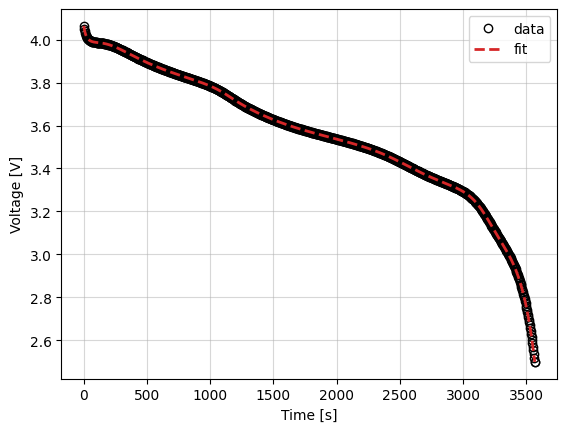
Now we use the callback object we created to plot the results at the end of the optimization.

_ = callback.plot_fit_results()

Cost logger

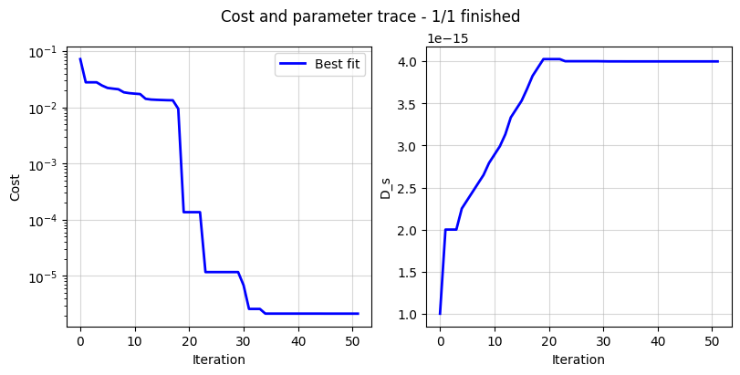
The DataFit class has an internal “cost-logger” attribute that can be used to log and visualize the cost function during optimization. This is useful for monitoring the progress of the optimization. The cost logger is a dictionary that stores the cost function value at each iteration. The cost logger can be accessed using the cost_logger attribute of the DataFit object.

By default, the cost logger tracks the cost function value. DataFit.plot_trace can be used the plot the progress at the end of the optimization.

objective = iwp.objectives.CurrentDriven(data, options={"model": model})
current_driven = iwp.DataFit(objective, parameters=parameters)
_ = current_driven.run(params_for_pipeline)
_ = current_driven.plot_trace()

[IDAS ERROR]  IDASolve
  At t = 0 and h = 8.88113e-60, the corrector convergence failed repeatedly or with |h| = hmin.

The cost logger can be changed by passing the cost_logger argument to the DataFit object. For example, the following example shows how to pass a cost logger that plots the cost function and parameter values every 10 seconds.

current_driven = iwp.DataFit(
    objective,
    parameters=parameters,
    cost_logger=iwp.data_fits.CostLogger(plot_every=10),
)