Combining Objectives example

This notebook shows how to construct and combine custom Objective classes to fit multiple objectives at once (e.g. simultaneously fit two data sets). For design principles, see the user_guide. For detailed documentation on the Objective class, see the API reference.

import pybamm
import numpy as np
import pandas as pd
import ionworkspipeline as iwp

Simple pulse example

For this example, we set up a single particle model with a temperature dependent diffusivity. The goal is to fit the activation energy of the diffusivity using data generated from simple pulse experiments conducted at different temperatures.

We first set up the model and parameters.

model = pybamm.lithium_ion.SPM()
parameter_values = iwp.ParameterValues("Chen2020")


def D_n(c, T):
    D_ref = pybamm.Parameter("Negative electrode reference diffusivity [m2.s-1]")
    E_D_s = pybamm.Parameter(
        "Negative particle diffusivity activation energy [J.mol-1]"
    )
    arrhenius = np.exp(-E_D_s / (pybamm.constants.R * T)) * np.exp(
        E_D_s / (pybamm.constants.R * 296)
    )
    return D_ref * arrhenius


parameter_values.update(
    {
        "Negative particle diffusivity [m2.s-1]": D_n,
        "Negative electrode reference diffusivity [m2.s-1]": 3.3e-14,
        "Negative particle diffusivity activation energy [J.mol-1]": 2.5e4,
    },
    check_already_exists=False,
)

Then we generate some synthetic data.

data_dict = {}
sols = []
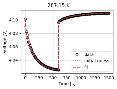
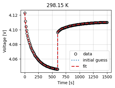
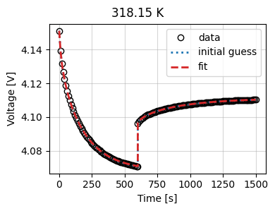
for T in [287.15, 298.15, 318.15]:
    parameters_for_data = parameter_values.copy()
    experiment = pybamm.Experiment(
        ["Discharge at C/3 for 10 minutes", "Rest for 15 minutes"],
        period="10 seconds",
        temperature=T,
    )
    sim = pybamm.Simulation(
        model, parameter_values=parameters_for_data, experiment=experiment
    )
    sim.solve()
    sols.append(sim.solution)
    data_dict[T] = pd.DataFrame(
        {x: sim.solution[x].entries for x in ["Time [s]", "Current [A]", "Voltage [V]"]}
    )

We can look at the data.

pybamm.dynamic_plot(
    sols, ["Current [A]", "Voltage [V]"], labels=[f"{T} K" for T in data_dict]
)

<pybamm.plotting.quick_plot.QuickPlot at 0x79a237953020>

Now we set up which parameters are to be fitted, and call the pre-defined CurrentDriven objective function, which solves the model with the current from the data and calculates the error between voltage from the model and the data. We can set up an objective for the data collected at each temperature, passing in the temperature using the custom_parameters argument of the objective function. Any values provided in the custom_parameter dictionary are passed the simulation in that objective only.

# In this example we fit both the reference diffusivity and activation energy in
# the negative electrode
parameters = {
    "Negative electrode reference diffusivity [m2.s-1]": iwp.Parameter(
        "D_ref", initial_value=1e-13, bounds=(1e-15, 1e-12)
    ),
    "Negative particle diffusivity activation energy [J.mol-1]": iwp.Parameter(
        "E_D_s", initial_value=1e4, bounds=(1e3, 1e5)
    ),
}

# We loop over the data at different temperatures, and create a separate objective
# for each temperature, storing them in a dictionary
objectives = {}
for T, data in data_dict.items():
    objectives[f"{T} K"] = iwp.objectives.CurrentDriven(
        data, options={"model": model}, custom_parameters={"Ambient temperature [K]": T}
    )

# We then create a data fit object, passing in the objectives and the parameters. This
# will fit the parameters to all data simultaneously
current_driven = iwp.DataFit(objectives, parameters=parameters)

# make sure we're not accidentally initializing with the correct values by passing
# them in
params_for_pipeline = {k: v for k, v in parameter_values.items() if k not in parameters}

results = current_driven.run(params_for_pipeline)

Let’s look at the results

for parameter in parameters:
    print(parameter)
    print(f"True parameter value: {parameter_values[parameter]:.3e}")
    print(f"Fitted parameter value: {results[parameter]:.3e}")

Negative electrode reference diffusivity [m2.s-1]
True parameter value: 3.300e-14
Fitted parameter value: 3.530e-14
Negative particle diffusivity activation energy [J.mol-1]
True parameter value: 2.500e+04
Fitted parameter value: 2.011e+03

_ = current_driven.plot_fit_results()