Fitting OCP hysteresis

In this example, we show how to fit the lithiation and delithiation OCPs at the same time in a way that is consistent with the MSMR model. In particular, we want the total capacity to be the same during lithiation and delithiation. To ensure this, we fit a single capacity for each species, but allow the reaction parameters \(X_j\), \(U0_j\) and \(\omega_j\) to be different for lithiation and delithiation.

import ionworkspipeline as iwp
import numpy as np
import pandas as pd
import matplotlib.pyplot as plt
from scipy.signal import savgol_filter

We use data from half-cells constructed from an LGM50 cell, as reported in https://github.com/paramm-team/pybamm-param.

data = {}
Q_max_data = 0
fig, ax = plt.subplots(1, 3, figsize=(10, 5))
for direction in ["lithiation", "delithiation"]:
    # Smooth
    raw_ocp_data = pd.read_csv(f"anode_ocp_{direction}.csv", comment="#")
    q_smoothed = savgol_filter(
        raw_ocp_data["Capacity [A.h]"].values, window_length=11, polyorder=1
    )
    U_smoothed = savgol_filter(
        raw_ocp_data["Voltage [V]"].values, window_length=11, polyorder=1
    )

    # Store in a dataframe
    ocp_data = pd.DataFrame({"Capacity [A.h]": q_smoothed, "Voltage [V]": U_smoothed})
    # Preprocess
    ocp_data = iwp.data_fits.preprocess.sort_capacity_and_ocp(ocp_data)
    ocp_data = iwp.data_fits.preprocess.remove_ocp_extremes(ocp_data)
    q = ocp_data["Capacity [A.h]"].values
    U = ocp_data["Voltage [V]"].values
    data[direction] = ocp_data
    # Maximum capacity, will be used later as an initial guess for the electrode capacity
    Q_max_data = max(Q_max_data, ocp_data["Capacity [A.h]"].max())

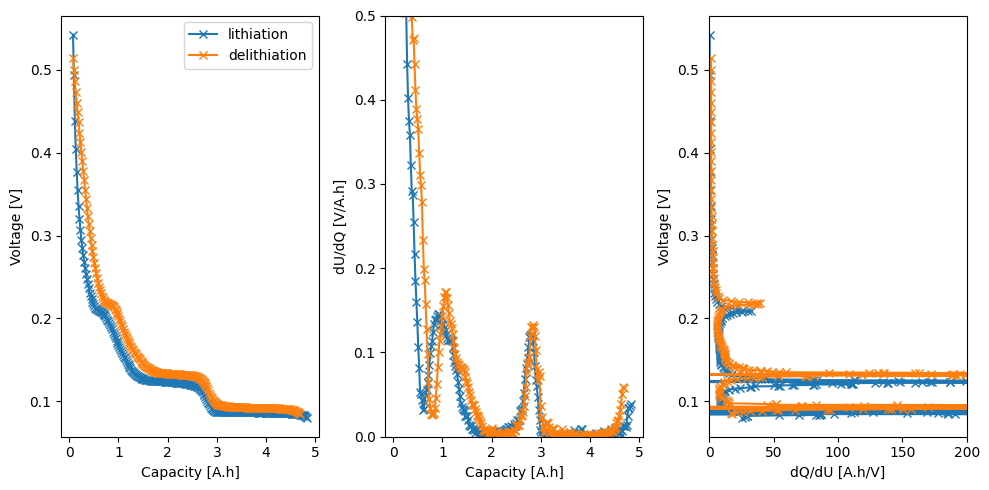
    # Plot
    dUdQ = -np.gradient(U, q)
    dQdU = -np.gradient(q, U)
    ax[0].plot(q, U, "-x", label=direction)
    ax[0].set_xlabel("Capacity [A.h]")
    ax[0].set_ylabel("Voltage [V]")
    ax[1].plot(q, dUdQ, "-x")
    ax[1].set_xlabel("Capacity [A.h]")
    ax[1].set_ylabel("dU/dQ [V/A.h]")
    ax[1].set_ylim(0, 0.5)
    ax[2].plot(dQdU, U, "-x")
    ax[2].set_xlabel("dQ/dU [A.h/V]")
    ax[2].set_ylabel("Voltage [V]")
    ax[2].set_xlim(0, 200)
ax[0].legend()
fig.tight_layout()

Next we set up the Parameter objects for the fit. For the reaction parameters, we use the values from Verbrugge et al 2017 J. Electrochem. Soc. 164 E3243 as an initial guess. We can access the values from the Material object, which is part of our library of parameter values.

We set up a bounds function that returns the bounds for the reaction parameters. Here we use the same bounds for lithiation and delithiation, and for each reaction index \(j\). We could construct a more complex bounds function that allows the bounds to be different for lithiation and delithiation, and/or different for each reaction index \(j\).

# Initial guess of Graphite from Verbrugge et al 2017 J. Electrochem. Soc. 164 E3243
msmr_param_init = iwp.Material("GRAPHITE_VERBRUGGE2017").parameter_values


# Define bounds for the MSMR parameters
def bounds_function(var, initial_value, Q_total):
    if var.startswith("X"):
        return 0, 1
    elif var.startswith("U"):
        return max(0, initial_value - 0.2), initial_value + 0.2
    elif var.startswith("w"):
        return 1e-2, 100
    else:
        raise ValueError(f"Unknown parameter {var}")

Now we create a dictionary of parameters to fit. We fit a single capacity for each species, but allow the lower excess capacity to be different for lithiation and delithiation, since the data in both directions may not span the same range of capacities. For the reaction parameters, we use the the helper function get_msmr_params_for_fit to create the Parameter objects.

params_to_fit = {
    "Negative electrode capacity [A.h]": iwp.Parameter(
        "Q_n", initial_value=Q_max_data, bounds=(Q_max_data * 0.8, Q_max_data * 1.2)
    ),
    "Negative electrode lower excess capacity (delithiation) [A.h]": iwp.Parameter(
        "Q_n_d_lowex", initial_value=0.01 * Q_max_data, bounds=(0, 0.1 * Q_max_data)
    ),
    "Negative electrode lower excess capacity (lithiation) [A.h]": iwp.Parameter(
        "Q_n_l_lowex", initial_value=0.01 * Q_max_data, bounds=(0, 0.1 * Q_max_data)
    ),
}
params_to_fit.update(
    {
        **iwp.objectives.get_msmr_params_for_fit(
            msmr_param_init,
            "negative",
            Q_max_data,
            bounds_function=bounds_function,
            species_format="Xj",
            hysteresis=True,
        )
    }
)

Next we create the objectives. For this fit, we use the OpenCircuitHalfCellHysteresisCallback that shows both the fit results on a single plot. We create a single instance of the callback and pass it to each objective.

objectives = {}
callback = iwp.objectives.OpenCircuitHalfCellHysteresisCallback()
for direction in ["lithiation", "delithiation"]:
    objectives[direction] = iwp.objectives.MSMRHalfCell(
        data[direction],
        options={
            "model": iwp.data_fits.models.MSMRHalfCellModel(
                "negative", options={"species format": "Xj", "direction": direction}
            ),
            "dUdQ cutoff": 0.2,
            "voltage limits": (0, 1),
        },
        callbacks=callback,
    )

Finally, we create the DataFit object, run the fit,

data_fit = iwp.DataFit(objectives, parameters=params_to_fit)

results = data_fit.run({"Ambient temperature [K]": 298.15})

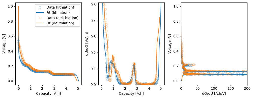
and plot the results.

fig, axes = callback.plot_fit_results()
_ = axes[2].set_xlim(0, 200)