Uncertainty quantification – Markov chain Monte Carlo Sampling

Step 1. Initial optimization

In this example, we will use Markov chain Monte Carlo (MCMC) sampling to quantify uncertainty in battery model parameters by fitting to synthetic data.

We begin by generating some synthetic data from a battery model.

import pybamm
import ionworkspipeline as iwp
import numpy as np
import pandas as pd

# Load the model and parameter values
model = pybamm.lithium_ion.SPM()
parameter_values = pybamm.ParameterValues("Chen2020")
parameter_values.update(
    {
        "Negative electrode active material volume fraction": 0.75,
        "Positive electrode active material volume fraction": 0.665,
    }
)

# Generate the data
t = np.linspace(0, 900, 1000)
sim = iwp.Simulation(
    model, parameter_values=parameter_values, t_eval=[0, 900], t_interp=t
)
sol = sim.solve()
data = pd.DataFrame(
    {x: sim.solution[x](t) for x in ["Time [s]", "Current [A]", "Voltage [V]"]}
)

In this example, we add normally distributed noise to the data. The standard deviation of the measurement error is important for uncertainty quantification, so this term is saved in a dictionary. The standard deviation of output variables can estimated after running an initial optimization.

# add noise to the data
V_sigma = 0.001
variable_standard_deviations = {"Voltage [V]": V_sigma}

np.random.seed(0)
data["Voltage [V]"] += np.random.normal(0, V_sigma, len(data))

Next, we define the parameters to fit, along with initial guesses and bounds.

parameters = {
    "Negative electrode active material volume fraction": iwp.Parameter(
        "Anode active material frac.",
        initial_value=0.5,
        bounds=(0, 1),
    ),
    "Positive electrode active material volume fraction": iwp.Parameter(
        "Cathode active material frac.",
        initial_value=0.5,
        bounds=(0, 1),
    ),
}

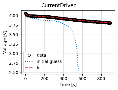
We set up the objective function, which in this case is the current driven objective. This takes the time vs current data and runs the model, comparing the model’s predictions for the voltage with the experimental data.

objective = iwp.objectives.CurrentDriven(data, options={"model": model})

Then, we set up the DataFit object, which takes the objective function and the parameters to fit as inputs.

data_fit = iwp.DataFit(objective, parameters=parameters, multistarts=10)

Next, we run the data fit, passing the parameters that are not being fit as a dictionary.

params_for_pipeline = {k: v for k, v in parameter_values.items() if k not in parameters}
results = data_fit.run(params_for_pipeline)
for k, v in results.items():
    print(f"{k}: {parameter_values[k]:.3e} (true) {v:.3e} (fit)")

Negative electrode active material volume fraction: 7.500e-01 (true) 7.513e-01 (fit)
Positive electrode active material volume fraction: 6.650e-01 (true) 6.646e-01 (fit)

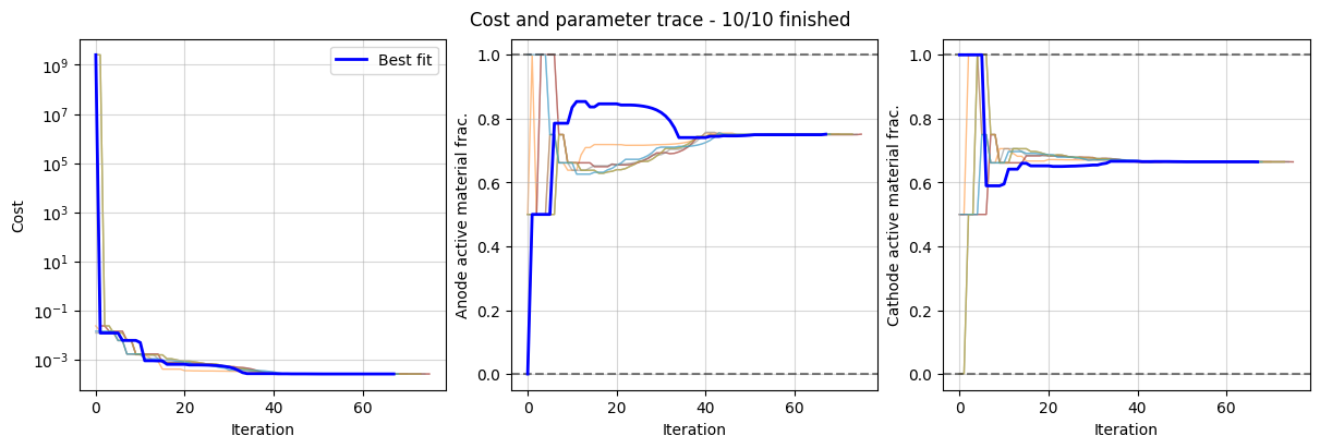
Finally, we plot the optimizer results and the trace of the cost function and parameter values.

_ = data_fit.plot_fit_results()
_ = data_fit.plot_trace()

Step 2. Uncertainty quantification

The Chi-square uncertainty quantification requires the output variables’ measurement error in order to provide a statistically meaningful confidence region. In this example, 0.001 V of error. In practice, this measurement error may not be known or there may be significant model-data mismatch. Using the results of the data_fit evaluation, we can estimate the variables’ standard deviation/

data_fit.estimate_variable_standard_deviations()

{'Voltage [V]': 0.0009864258852471683}

Which closely matches the known standard deviation of 0.001 V.

Using the data_fit results and the standard deviation, we can get a rough linear estimate for the confidence intervals.

confidence_intervals_linear = data_fit.linear_confidence_intervals(
    confidence_level=0.95,
    variable_standard_deviations=variable_standard_deviations,
    use_parameter_bounds=False,
)

for k, (lb, ub) in confidence_intervals_linear.items():
    print(f"{k}: {lb:.4f}, {ub:.4f}")

Negative electrode active material volume fraction: 0.7481, 0.7545
Positive electrode active material volume fraction: 0.6640, 0.6652

Now, we can perform the Chi-square uncertainty quantification. For this example, we use the Pints sampler which is an MCMC sampler. For performance, we tighten the bounds of the parameters to fit. The ChiSquare cost requires the variable_standard_deviations to generate statistically significant parameter bounds.

parameters_tight_bounds = {
    "Negative electrode active material volume fraction": iwp.Parameter(
        "Anode active material frac.",
        bounds=(0.7471, 0.7554),
    ),
    "Positive electrode active material volume fraction": iwp.Parameter(
        "Cathode active material frac.",
        bounds=(0.6637, 0.6654),
    ),
}

sampler_fit = iwp.DataFit(
    objective,
    cost=iwp.costs.ChiSquare(variable_standard_deviations),
    optimizer=iwp.samplers.Pints(max_iterations=800),
    multistarts=10,
    options={"seed": 0},
    parameters=parameters_tight_bounds,
)

sampler_fit.run(params_for_pipeline)

Result(
  Negative electrode active material volume fraction: 0.751403
  Positive electrode active material volume fraction: 0.664566
)

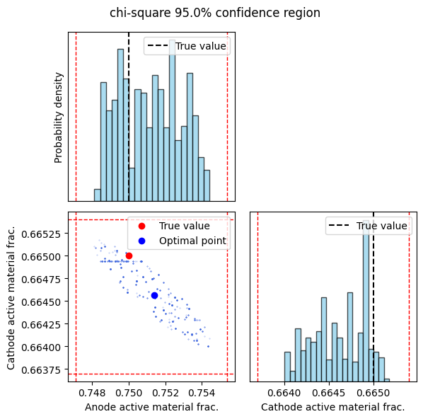
The sampler_results function visualizes the results of the MCMC sampling and calculates confidence intervals. It creates a corner plot showing the marginal distributions of each parameter and their joint distribution. The true parameter values are overlaid on the plots for comparison. The function also prints and returns the confidence intervals at the specified confidence level.

def sampler_results(sampler_fit, confidence_level):
    fig, axes = sampler_fit.plot_sampler_results(
        confidence_level=confidence_level, bins=20
    )

    names = [
        "Negative electrode active material volume fraction",
        "Positive electrode active material volume fraction",
    ]
    true_values = [parameter_values[k] for k in names]
    # Plot the true values. Axes is a list of lists of axes
    for i, v in enumerate(true_values):
        ax = axes[i][i]
        ax.axvline(v, color="k", linestyle="--", label="True value")
        ax.legend(loc="upper right")

    ax = axes[-1][0]
    ax.scatter(true_values[0], true_values[1], color="red", label="True value")
    optimal_point = [sampler_fit.results.parameter_values[name] for name in names]
    ax.scatter(optimal_point[0], optimal_point[1], color="blue", label="Optimal point")
    ax.legend(loc="upper right")

    fig.set_figheight(6)
    fig.set_figwidth(6)
    fig.tight_layout()
    confidence_intervals = sampler_fit.sampler_confidence_intervals(
        confidence_level=confidence_level
    )
    print(f"Confidence level: {confidence_level}")
    for k, (lb, ub) in confidence_intervals.items():
        print(f"{k}: {lb:.4f}, {ub:.4f}")

    return confidence_intervals


_ = sampler_results(sampler_fit, confidence_level=0.95)

Confidence level: 0.95
Negative electrode active material volume fraction: 0.7481, 0.7544
Positive electrode active material volume fraction: 0.6640, 0.6652

_ = sampler_results(sampler_fit, confidence_level=0.99)

Confidence level: 0.99
Negative electrode active material volume fraction: 0.7474, 0.7553
Positive electrode active material volume fraction: 0.6639, 0.6653

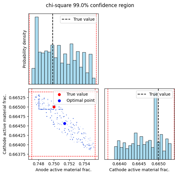
The confidence_level can be adjusted to determine other parameter confidence intervals. The full-order sampling confidence intervals are close to the values approximated by linearizing the model. As expected, the 99% confidence region is larger than the 95% confidence region as it contains more point estimates. In both cases, the true values of the anode and cathode volume fractions are contained within the confidence intervals, however, this may not always be the case with nonlinear battery models.