Exchange-current density from resistance

In this example, we show how to fit the exchange-current density to resistance data calculated from synthetic pulse data.

import pybamm
import ionworkspipeline as iwp
import pandas as pd

We begin by generating synthetic pulse data for a half-cell. We use the standard symmetric exchange-current density function and will fit the reference value. We set up the model and parameters,

model = pybamm.lithium_ion.SPMe(
    {"working electrode": "positive", "particle": "uniform profile"}
)
model.events = []
parameter_values = iwp.ParameterValues("Xu2019")


def j0(c_e, c_s_surf, c_s_max, T):
    j0_ref = pybamm.Parameter(
        "Positive electrode reference exchange-current density [A.m-2]"
    )
    c_e_init = pybamm.Parameter("Initial concentration in electrolyte [mol.m-3]")

    return (
        j0_ref
        * (c_e / c_e_init) ** 0.5
        * (c_s_surf / c_s_max) ** 0.5
        * (1 - c_s_surf / c_s_max) ** 0.5
    )


parameter_values.update(
    {
        "Positive electrode reference exchange-current density [A.m-2]": 5,
        "Positive electrode exchange-current density [A.m-2]": j0,
    },
    check_already_exists=False,
)

and then simulate a GITT experiment.

C_rate = 1 / 15
pause_s = 10  # 10s
step_s = 5 * 60  # 5m
step_h = step_s / 3600
rest_s = 1 * 3600  # 1h
max_cycles = int(1 / C_rate / step_h * 2)
V_min = parameter_values["Lower voltage cut-off [V]"]

gitt_experiment = pybamm.Experiment(
    [
        (
            pybamm.step.rest(pause_s, period=1),
            pybamm.step.c_rate(
                C_rate,
                duration=step_s,
                period=step_s / 100,
                termination=f"{V_min} V",
            ),
            pybamm.step.rest(rest_s, period=rest_s / 100),
        ),
    ]
)
sim = iwp.Simulation(
    model, parameter_values=parameter_values, experiment=gitt_experiment
)
sol = None
i = 0

# Run until the voltage drops below the lower cut-off
# during step 1 (the discharge step)
while sol is None or sol.cycles[-1].steps[1].termination == "final time":
    sol = sim.solve(starting_solution=sol)
    i += 1
    if i > max_cycles:
        raise ValueError("Reached maximum number of cycles")

We export the solution data to a dataframe.

Note: for synthetic data we can directly store the stoichiometry, whereas in practice we would need to compute this from the half-cell capacity and the charge passed.

variables = [
    "Time [s]",
    "Current [A]",
    "Voltage [V]",
    "Positive electrode stoichiometry",
]
df = pd.DataFrame(sim.solution.get_data_dict(variables))
df = df.rename(columns={"Cycle": "Cycle number", "Step": "Step number"})

Next we calculate the 1s resistance from the solution data using the function iwp.objectives.pulse.calculate_pulse_resistance. We pass in the step number “1” which is the “on” step of our pulse data (steps 0 and 2 are the “off” steps).

steps = [1]
dts = [1]
data = iwp.objectives.pulse.calculate_pulse_resistance("positive", df, steps, dts)

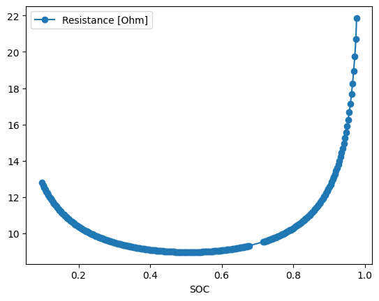
We can then plot the calculated resistance as a function of stoichiometry.

_ = data.plot(x="SOC", y="Resistance [Ohm]", style="o-")

Next, we set up the objective that will be used to perform the fit.

model = iwp.objectives.HalfCellResistanceModel("positive")
objective = iwp.objectives.Resistance(data, {"model": model})

We fit the exchange-current density and an extra scalar “contact resistance” parameter that accounts for any other resistances.

parameters = {
    "Positive electrode reference exchange-current density [A.m-2]": iwp.Parameter(
        "j0_ref", initial_value=1, bounds=(0.1, 10)
    ),
    "Contact resistance [Ohm]": iwp.Parameter("R_contact"),
}
data_fit = iwp.DataFit(objective, parameters=parameters)

We pass in the known parameter values and run the fit.

# make sure we're not accidentally initializing with the correct values by passing
# them in
params_for_pipeline = {k: v for k, v in parameter_values.items() if k not in parameters}
data_fit.run(params_for_pipeline)

Result(
  Positive electrode reference exchange-current density [A.m-2]: 5.04718
  Contact resistance [Ohm]: 2.6453
)

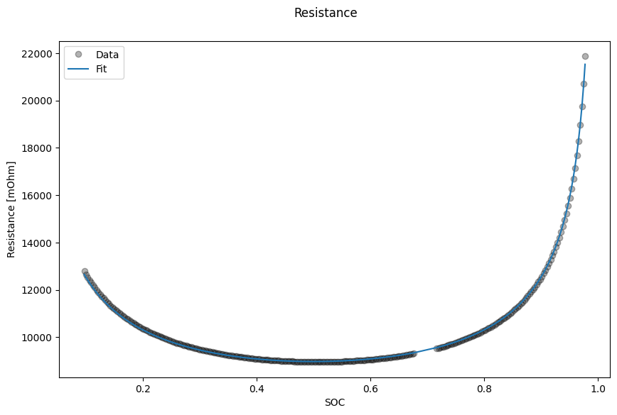
Finally, we plot the results.

_ = data_fit.plot_fit_results()