2. Full-cell OCV

In this example, we use synthetic full-cell GITT data and known half-cell OCP parameters to determine the stoichiometry windows that give the correct full-cell OCV, a process often referred to as “electrode balancing”.

Before running this example, make sure to run the script true_parameters/generate_data.py to generate the synthetic data.

from pathlib import Path

import ionworkspipeline as iwp
import iwutil

from true_parameters.parameters import get_msmr_parameters

Cell balancing theory

Given the open-circuit potentials for each electrode, we combine them to get the full-cell open-circuit voltage

\[U_{cell}(z) = U_{p}(\theta_{p}) - U_{n}(\theta_{n}),\]

where \(z\) is the full-cell state of charge, and \(\theta_{n}\) and \(\theta_{p}\) are the electrode-level state of charge of the negative and positive electrodes respectively (usually called “stoichiometry” or “lithiation” to avoid confusion with cell-level state of charge). To evaluate the OCV, we need to convert the stoichiometry of each electrode to the full-cell state of charge. This is done using the following formula:

\[ z = \frac{\theta_{n} - \theta_{n}^\mathrm{0}}{\theta_{n}^\mathrm{100} - \theta_{n}^\mathrm{0}} = \frac{\theta_{p} - \theta_{p}^\mathrm{0}}{\theta_{p}^\mathrm{100} - \theta_{p}^\mathrm{0}}, \]

where \(\theta_{n}^\mathrm{0}\), \(\theta_{n}^\mathrm{100}\), \(\theta_{p}^\mathrm{0}\), \(\theta_{p}^\mathrm{100}\) are the stoichiometries of the negative and positive electrodes at 0% and 100% state of charge respectively. Hence the challenge is to find the four values \(\theta_{n}^\mathrm{0}\), \(\theta_{n}^\mathrm{100}\), \(\theta_{p}^\mathrm{0}\), \(\theta_{p}^\mathrm{100}\), that best fit the full-cell open-circuit voltage data. In practice, full-cell OCV data is is given in terms of capacity instead of stoichiometry. Therefore, we reformulate the full-cell open-circuit voltage as a function of capacity:

\[U_{cell}(q) = U_{p}(q_{p}) - U_{n}(q_{n}),\]

where \(q = Qz\), \(q_{n} = \theta_{n}Q_{n}\), \(q_{p} = \theta_{p}Q_{p}\), and \(Q\) is the total capacity of the cell and \(Q_{n}\) and \(Q_{p}\) are the total capacities of the individual electrodes. We can then convert between the full-cell capacity and the electrode capacities using the following formula:

\[ q/Q = \frac{q_{n} - q_{n}^\mathrm{0}}{q_{n}^\mathrm{100} - q_{n}^\mathrm{0}} = \frac{q_{p} - q_{p}^\mathrm{0}}{q_{p}^\mathrm{100} - q_{p}^\mathrm{0}}. \]

We find the values of \(q_{n}^\mathrm{0}\), \(q_{n}^\mathrm{100}\), \(q_{p}^\mathrm{0}\), \(q_{p}^\mathrm{100}\) that best fit the data.

In this example, we fit the “lower excess capacity” and “upper excess capacity” instead of the stoichiometries at 0% and 100% state of charge. We use these names because the data typically does not reach the true 0% and 100% state of charge, due to kinetic limitations and/or electrolyte stability. The lower excess capacity is equal to \(q_{n}^\mathrm{0}\) in the negative electrode, and \(q_{p}^\mathrm{100}\) in the positive electrode. The upper excess capacity is equal to \(Q_{n} - q_{n}^\mathrm{100}\) in the negative electrode, and \(Q_{p} - q_{p}^\mathrm{0}\) in the positive electrode. \(Q\) is given by the actual total capacity observed in the experimental data (called “useable capacity” in the example).

Load the data

We load the synthetic GITT data and the extract the OCP from the relaxed voltages.

gitt_data = iwutil.read_df(Path("synthetic_data") / "full_cell" / "gitt.csv")
ocp_data = iwp.data_fits.preprocess.pulse_data_to_ocp(gitt_data)

Get the known parameters

In this example, we assume we already know the MSMR OCP parameters for the negative and positive electrodes. In practice, these parameters can be fitted using the half-cell OCV workflow.

msmr_params_n = get_msmr_parameters("negative")
msmr_params_p = get_msmr_parameters("positive")
known_params = {
    **msmr_params_n,
    **msmr_params_p,
    "Ambient temperature [K]": 298.15,
}

Set up the parameters to fit

Now we set up our initial guesses for the parameters. As in the previous example, we create a dictionary of Parameter objects.

Q_use = ocp_data["Capacity [A.h]"].max()
Q_n_lowex = iwp.Parameter(
    "Q_n_lowex", initial_value=0.01 * Q_use, bounds=(0, 0.2 * Q_use)
)
Q_p_lowex = iwp.Parameter("Q_p_lowex", initial_value=0.1 * Q_use, bounds=(0, Q_use))
Q_n_uppex = iwp.Parameter(
    "Q_n_uppex", initial_value=0.1 * Q_use, bounds=(0, 0.2 * Q_use)
)
Q_p_uppex = iwp.Parameter("Q_p_uppex", initial_value=0.5 * Q_use, bounds=(0, Q_use))
parameters = {
    "Negative electrode lower excess capacity [A.h]": Q_n_lowex,
    "Positive electrode lower excess capacity [A.h]": Q_p_lowex,
    "Negative electrode upper excess capacity [A.h]": Q_n_uppex,
    "Positive electrode upper excess capacity [A.h]": Q_p_uppex,
    "Negative electrode capacity [A.h]": Q_n_lowex + Q_use + Q_n_uppex,
    "Positive electrode capacity [A.h]": Q_p_lowex + Q_use + Q_p_uppex,
    "Usable capacity [A.h]": Q_use,
}

Run the workflow

Now we are ready to run the workflow. To run the workflow with the default settings, we can use the fit_plot_save function. This function runs the fit, saves the results (if a save_dir keyword argument is provided), and plots the results. All of the workflows have a common interface, where you typically need to provide the data, the parameters to be fitted, and a dictionary of known parameters.

For the full-cell OCV workflow, we need to specify the voltage range of each electrode to use in the fit. We can do this by passing a dictionary of keyword arguments, objective_kwargs, to be used in the objective. The limits are used to evaluate the half-cell OCPs in the fit, and should therefore span a wider half-cell voltage range than we expect to see in the data.

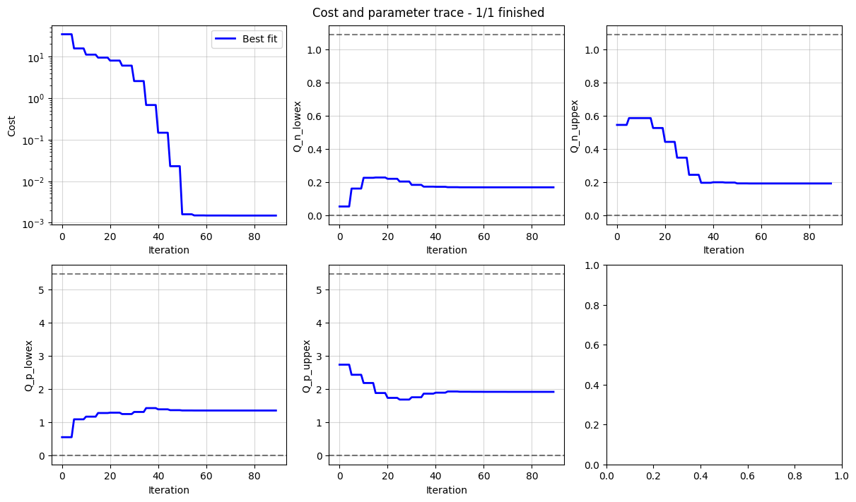
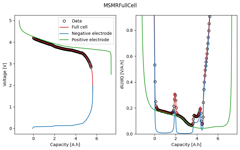
The workflow returns a Results object, which contains the fitted parameters, and a dictionary of figures with the keys “trace” and the name of the objective function (in this case “MSMRFullCell”). The trace figure shows the evolution of the cost function and parameter values during the fit. The MSMRFullCell figure shows the fitted OCV and dU/dQ curves. In the plot, we can see how the half-cell OCPs combine to give the full-cell OCV.

options = {
    # these are the voltage ranges over which to evaluate the half-cell OCP curves
    "negative voltage limits": (0, 2),
    "positive voltage limits": (2.5, 5),
}
objective_kwargs = {
    "options": options,
}
res, figs = iwp.workflows.full_cell_ocv.fit_plot_save(
    ocp_data,
    parameters,
    known_params,
    objective_kwargs=objective_kwargs,
)

We can take a look at the fitted parameters by accessing the parameter_values attribute of the Results object.

res.parameter_values

{'U0_n_0': 0.08466942669348111,
 'X_n_0': 0.30203768678220166,
 'w_n_0': 0.12716880189789798,
 'U0_n_1': 0.13066249665852994,
 'X_n_1': 0.26549403517199244,
 'w_n_1': 0.03977295676305788,
 'U0_n_2': 0.1573326877633104,
 'X_n_2': 0.15380340586780292,
 'w_n_2': 0.8965366857551075,
 'U0_n_3': 0.21983989110917385,
 'X_n_3': 0.1113636714034817,
 'w_n_3': 4.061201551170516,
 'U0_n_4': 0.21555155560469588,
 'X_n_4': 0.03207477786300497,
 'w_n_4': 0.060001175656655,
 'U0_n_5': 0.5495549372260156,
 'X_n_5': 0.13522669968702852,
 'w_n_5': 8.401333270326665,
 'Ambient temperature [K]': 298.15,
 'U0_p_0': 3.62274,
 'X_p_0': 0.13442,
 'w_p_0': 0.9671,
 'U0_p_1': 3.72645,
 'X_p_1': 0.3246,
 'w_p_1': 1.39712,
 'U0_p_2': 3.90575,
 'X_p_2': 0.21118,
 'w_p_2': 3.505,
 'U0_p_3': 4.22955,
 'X_p_3': 0.3298,
 'w_p_3': 5.52757,
 'Negative electrode lower excess capacity [A.h]': 0.17026546680704202,
 'Positive electrode lower excess capacity [A.h]': 1.3504646916622283,
 'Negative electrode upper excess capacity [A.h]': 0.19325686273682535,
 'Positive electrode upper excess capacity [A.h]': 1.9147839287729518,
 'Negative electrode capacity [A.h]': 5.827847531224868,
 'Positive electrode capacity [A.h]': 8.729573822116182,
 'Usable capacity [A.h]': 5.464325201681001,
 'Negative electrode lithiation': functools.partial(<function _theta_half_cell at 0x7c4a47f1d260>, 6, 'negative', 'Xj', None, False),
 'Positive electrode lithiation': functools.partial(<function _theta_half_cell at 0x7c4a47f1d260>, 4, 'positive', 'Xj', None, False),
 'Negative electrode stoichiometry at minimum SOC': 0.029215840993571166,
 'Negative electrode stoichiometry at maximum SOC': 0.9668390667907183,
 'Positive electrode stoichiometry at minimum SOC': 0.7806555087578401,
 'Positive electrode stoichiometry at maximum SOC': 0.15469995662799207}

What’s going on? A lower-level interface

The workflows are designed to be simple to use and cover most use cases. They can be customized by passing additional keyword arguments. For example, we can pass a dictionary datafit_kwargs to specify the cost function or optimizer to be used in the fit. Much more customization is possible by accessing the underlying DataFit and Optimizer classes directly. Here we will go through the steps of running the fit manually.

We can use the same parameters and known_params as dicitonaries as before, but we need to create the Objective and DataFit objects manually.

Let’s start by creating the objective function. We use the MSMRFullCell objective function and pass in the data and voltage limits.

objective = iwp.objectives.MSMRFullCell(
    ocp_data,
    options={
        "negative voltage limits": (0, 2),
        "positive voltage limits": (2.5, 5),
    },
)

After we’ve created the objective, we can create the DataFit object. The DataFit object takes in the objective and the parameters to fit. We can also customize the fitting processing by passing in a cost function and selecting an optimizer.

cost = iwp.costs.Difference()
optimizer = iwp.optimizers.ScipyLeastSquares(verbose=1)
datafit = iwp.DataFit(objective, parameters=parameters, cost=cost, optimizer=optimizer)

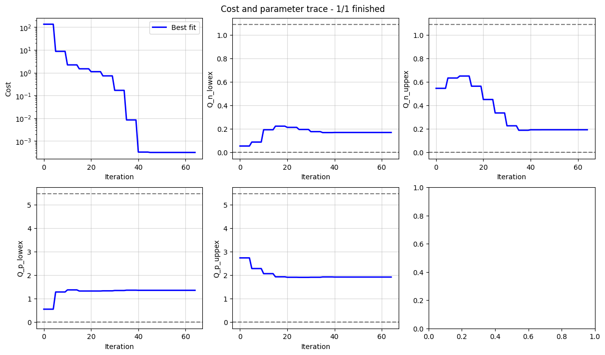
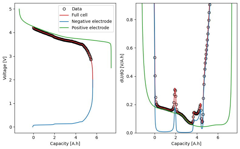
Finally, we run the fit and plot the results.

results = datafit.run(known_params)
_ = datafit.plot_trace()
_ = datafit.plot_fit_results()

`ftol` termination condition is satisfied.
Function evaluations 18, initial cost 1.7282e+01, final cost 7.3939e-04, first-order optimality 1.14e-06.