Cycle ageing example

This notebook demonstrates how to use the CycleAgeing objective function to fit the SEI solvent diffusivity in the “solvent-diffusion limited” SEI model using synthetic cycling data.

import pybamm
import ionworkspipeline as iwp
import pandas as pd

We begin by generating some synthetic cycling data. We choose the SPMe model and the “solvent-diffusion limited” SEI model and simulate 10 cycles of a CCCV charge/discharge cycle. For the data, we record the cycle number, the loss of lithium inventory, and the capacity. We choose the parameter values so that we get a large loss of lithium inventory even after only 10 cycles.

model = pybamm.lithium_ion.SPMe({"SEI": "solvent-diffusion limited"})
parameter_values = iwp.ParameterValues("Chen2020")
parameter_values.update(
    {
        "SEI solvent diffusivity [m2.s-1]": 2.5e-18,
    }
)

experiment = pybamm.Experiment(
    [
        (
            "Discharge at 1C until 2.5 V",
            "Rest for 1 hour",
            "Charge at C/2 until 4.2 V",
            "Hold at 4.2 V until 10 mA",
            "Rest for 1 hour",
        ),
    ]
    * 10
)

sim = iwp.Simulation(
    model,
    experiment=experiment,
    parameter_values=parameter_values,
)

sol = sim.solve()

data = {"Cycle number": sol.summary_variables.cycle_number}
for var in ["Loss of lithium inventory [%]", "Capacity [A.h]"]:
    data[var] = sol.summary_variables[var]

# PyBaMM uses 1-based indexing for cycles but ionworks data format assumes cycles number
# starts at zero
data["Cycle number"] = data["Cycle number"] - 1

data = pd.DataFrame(data)

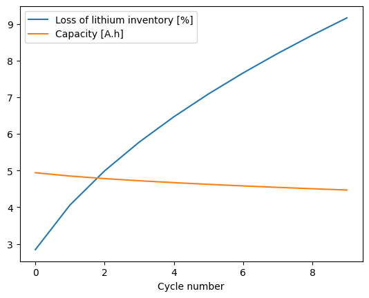
We can plot the synthetic data to see what it looks like.

_ = data.plot(
    x="Cycle number", y=["Loss of lithium inventory [%]", "Capacity [A.h]"], kind="line"
)

Next, we create the objective function. We pass the data and the options to the CycleAgeing objective function. The options include the model, experiment, and the objective variables (i.e. the variables we want to fit to). The CycleAgeing objective runs the experiment and calculates the cycling data. By default, it uses the function ionworkspipeline.data_fits.objectives.get_standard_summary_variables to extract the summary variables from the solution. Custom summary variables can be used by passing a custom function to the cycle_variables_function option.

objective = iwp.objectives.CycleAgeing(
    data,
    options={
        "model": model,
        "experiment": experiment,
        "objective variables": ["Loss of lithium inventory [%]"],
    },
)

We then create the data fit. We pass the objective function and the parameters to the DataFit class. The parameters include the initial values and bounds for the parameters we want to fit.

parameters = {
    "SEI solvent diffusivity [m2.s-1]": iwp.Parameter(
        "SEI solvent diffusivity [m2.s-1]",
        initial_value=1e-19,
        bounds=(1e-21, 1e-17),
    )
}
data_fit = iwp.DataFit(objective, parameters=parameters)

Next, we run the data fit. We pass the known parameters (i.e. those we are not fitting) to the data fit.

known_parameters = {k: v for k, v in parameter_values.items() if k not in parameters}
data_fit.run(known_parameters)

Result(
  SEI solvent diffusivity [m2.s-1]: 2.5e-18
)

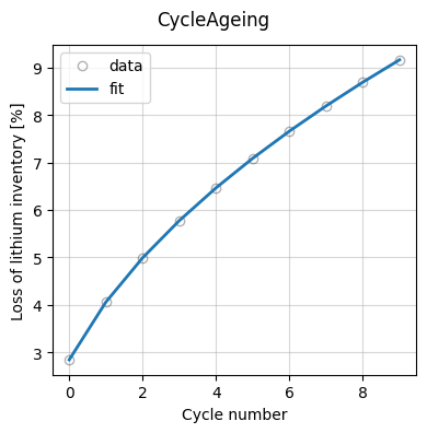
Finally, we plot the fit results.

_ = data_fit.plot_fit_results()