Fitting Arrhenius relationships to data

This example shows how to fit Arrhenius relationships to data using the ArrheniusLogLinear class.

We plan on adding more thermal functions in the future, so keep an eye out for updates!

import ionworkspipeline as iwp
import matplotlib.pyplot as plt
import pybamm
import pandas as pd
import numpy as np

Begin by generating some synthetic data.

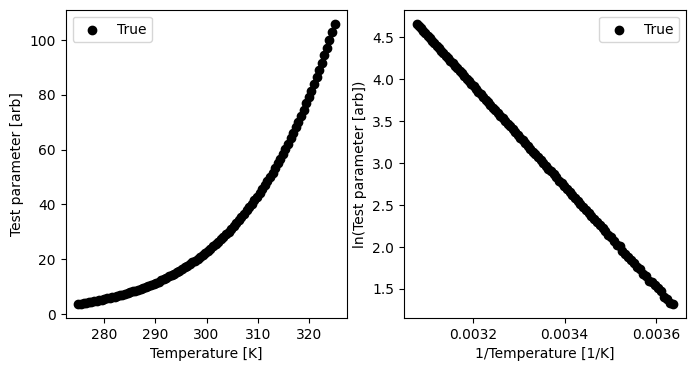
We will show this with a test parameter with units [arb], but this could be any parameter. The units are used to process the results. We add a bit of noise to the data to make it interesting.

R = pybamm.constants.R.value
T = np.linspace(275, 325, 100)
Ea_true = 50000.0
A_true = 20.0
T_ref = 298.15

param_name = "Test parameter [arb]"

param_val = A_true * np.exp(
    -Ea_true / (R * T) + Ea_true / (R * T_ref)
) + np.random.normal(0, 5e-2, len(T))

fig, ax = plt.subplots(1, 2, figsize=(8, 4))
ax[0].scatter(T, param_val, label="True", color="black")
ax[1].scatter(1 / T, np.log(param_val), label="True", color="black")
ax[0].set_xlabel("Temperature [K]")
ax[0].set_ylabel(param_name)
ax[1].set_xlabel("1/Temperature [1/K]")
ax[1].set_ylabel("ln(" + param_name + ")")
ax[0].legend()
ax[1].legend()

<matplotlib.legend.Legend at 0x7a2e4a4d3f20>

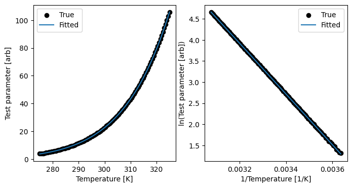
Now, we can fit the Arrhenius relationship using the ArrheniusLogLinear class provided by ionworkspipeline. The class takes as input a pandas DataFrame with the temperature and the parameter of interest. The reference temperature is optional, and if not provided, no reference temperature is used in the fit. Running the fit returns a dict with the activation energy, the pre-exponential factor (A), the reference temperature if provided, and a function for the parameter as a function of temperature.

arrh_fitter = iwp.calculations.ArrheniusLogLinear(
    pd.DataFrame({"Temperature [K]": T, param_name: param_val}),
    reference_temperature=T_ref,
)
param_values = arrh_fitter.run(None)
print(
    "Pre-exponential factor for test parameter [arb]:",
    param_values["Pre-exponential factor for test parameter [arb]"],
)
print("True pre-exponential factor for test parameter [arb]:", A_true)
print(
    "Activation energy for test parameter [J.mol-1]:",
    param_values["Activation energy for test parameter [J.mol-1]"],
)
print("True activation energy for test parameter [J.mol-1]:", Ea_true)
print("\n")
print("Full dict of results:")
print(param_values)


ax[0].plot(T, param_values["Test parameter [arb]"](T), label="Fitted")
ax[1].plot(
    1 / T, [np.log(param_values["Test parameter [arb]"](t)) for t in T], label="Fitted"
)
ax[0].legend()
ax[1].legend()
fig

Pre-exponential factor for test parameter [arb]: 19.987794396538558
True pre-exponential factor for test parameter [arb]: 20.0
Activation energy for test parameter [J.mol-1]: 50028.226051098216
True activation energy for test parameter [J.mol-1]: 50000.0


Full dict of results:
{'Activation energy for test parameter [J.mol-1]': 50028.226051098216, 'Test parameter [arb]': <function ArrheniusLogLinear.run.<locals>.<lambda> at 0x7a2e48942ca0>, 'Reference temperature for test parameter [K]': 298.15, 'Pre-exponential factor for test parameter [arb]': 19.987794396538558}

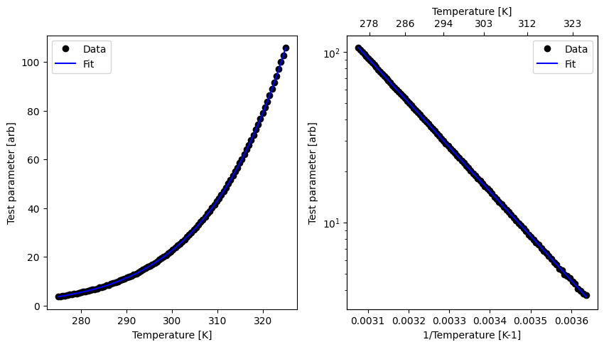
We also provide a plot_arrhenius method that plots the Arrhenius relationship once the calculation has been run.

fig, ax = arrh_fitter.plot_arrhenius()